Regression, 回归问题

Refer to http://www.r-tutor.com/elementary-statistics/simple-linear-regression

simple linear regression

A simple linear regression model that describes the relationship between two variables x and y can be expressed by the following equation. The numbers α and β are called parameters, and ϵ is the error term.

For example, in the data set faithful, it contains sample data of two random variables named waiting and eruptions. The waiting variable denotes the waiting time until the next eruptions, and eruptions denotes the duration. Its linear regression model can be expressed as:

线性回归是利用数理统计中的回归分析，来确定两种或两种以上变量间相互依赖的定量关系的一种统计分析方法之一，运用十分广泛。分析按照自变量和因变量之间的关系类型，可分为线性回归分析和非线性回归分析。

Estimated Simple Regression Equation, 简单回归方程式的预估

If we choose the parameters α and β in the simple linear regression model so as to minimize the sum of squares of the error term ϵ, we will have the so called estimated simple regression equation. It allows us to compute fitted values(拟合值) of y based on values of x.

Problem

Apply the simple linear regression model for the data set faithful, and estimate the next eruption duration if the waiting time since the last eruption has been 80 minutes.

根据已有的样本, 来预测下次喷发的时间

Solution

We apply the lm function to a formula that describes the variable eruptions by the variable waiting, andsave the linear regression model in a new variable eruption.lm.

> eruption.lm = lm(eruptions ~ waiting, data=faithful)

Then we extract the parameters of the estimated regression equation with the coefficients function.

> coeffs = coefficients(eruption.lm); coeffs  
(Intercept)     waiting  
-1.874016    0.075628

We now fit the eruption duration using the estimated regression equation.

> waiting = 80           # the waiting time  
> duration = coeffs[1] + coeffs[2]*waiting  
> duration  
(Intercept)  
     4.1762

Answer

Based on the simple linear regression model, if the waiting time since the last eruption has been 80 minutes, we expect the next one to last 4.1762 minutes.

Coefficient of Determination, 确定系数

The coefficient of determination of a linear regression model is the quotient of the variances of the fitted values and observed values of the dependent variable. If we denote y_i as the observed values of the dependent variable,  as its mean, and  as the fitted value, then the coefficient of determination is:

用来衡量, 拟合值(预测值)和观测值(真值)之间的差异, 说白了, 就是看看线性回归假设准不准...

Problem

Find the coefficient of determination for the simple linear regression model of the data set faithful.

Solution

We apply the lm function to a formula that describes the variable eruptions by the variable waiting, and save the linear regression model in a new variable eruption.lm.

> eruption.lm = lm(eruptions ~ waiting, data=faithful)

Then we extract the coefficient of determination from the r.squared attribute of its summary.

> summary(eruption.lm)$r.squared  
[1] 0.81146

Answer

The coefficient of determination of the simple linear regression model for the data set faithful is 0.81146.

Significance Test for Linear Regression, 线性回归的显著性测试

Assume that the error term ϵ in the linear regression model is independent of x, and is normally distributed, with zero mean and constant variance. We can decide whether there is any significant relationship between x and y by testing the null hypothesis that β = 0.

什么叫显著性测试, 说白了, 你假设的这个线性关系是否是真实存在的, 是否是牵强的,是否压根就没关系.

对于x = a+ by,  如果b可能为0, 那么x就是个常量, 和y就没啥关系.

所以对于这个线性回归, b为0一定是个小概率事件, 否则这个线性回归假设就不成立.

Note, 显著性检验的基本思想可以用小概率原理来解释. 小概率原理, 小概率事件在一次试验中是几乎不可能发生的, 假若在一次试验中事件事实上发生了. 那只能认为我们对总体所做的假设不正确.

所以这儿是个假设检验问题, testing the null hypothesis that β = 0, 如果这个假设不成立, 则此线性回归为显著的.

Problem

Decide whether there is a significant relationship between the variables in the linear regression model of the data set faithful at .05 significance level.

Solution

We apply the lm function to a formula that describes the variable eruptions by the variable waiting, and save the linear regression model in a new variable eruption.lm.

> eruption.lm = lm(eruptions ~ waiting, data=faithful)

Then we print out the F-statistics of the significance test with the summary function.

> summary(eruption.lm)  

Call:  
lm(formula = eruptions ~ waiting, data = faithful)  

Residuals:  
    Min      1Q  Median      3Q     Max  
-1.2992 -0.3769  0.0351  0.3491  1.1933  

Coefficients:  
            Estimate Std. Error t value Pr(>|t|)  
(Intercept) -1.87402    0.16014   -11.7   <2e-16 *** 
waiting      0.07563    0.00222    34.1   <2e-16 *** 
--- 
Signif. codes:  0 ’***’ 0.001 ’**’ 0.01 ’*’ 0.05 ’.’ 0.1 ’ ’ 1  

Residual standard error: 0.497 on 270 degrees of freedom  
Multiple R-squared: 0.811,      Adjusted R-squared: 0.811  
F-statistic: 1.16e+03 on 1 and 270 DF,  p-value: <2e-16

Answer

As the p-value is much less than 0.05, we reject the null hypothesis that β = 0. Hence there is a significant relationship between the variables in the linear regression model of the data set faithful.

我没看懂过程, 总之结果是reject null hypothesis

Confidence Interval for Linear Regression, 线性回归的置信区间

Assume that the error term ϵ in the linear regression model is independent of x, and is normally distributed, with zero mean and constant variance. For a given value of x, the interval estimate for the mean of the dependent variable,  , is called the confidence interval.

看例子就知道了, 回归是预测, 所以不可能完全精准, 所以给出一个置信区间比给一个单值更为合理. 之所以叫置信区间, 因为区间的范围是基于置信度的.

Problem

In the data set faithful, develop a 95% confidence interval of the mean eruption duration for the waiting time of 80 minutes.

Solution

We apply the lm function to a formula that describes the variable eruptions by the variable waiting, and save the linear regression model in a new variable eruption.lm.

> attach(faithful)     # attach the data frame  
> eruption.lm = lm(eruptions ~ waiting)

Then we create a new data frame that set the waiting time value.

> newdata = data.frame(waiting=80)

We now apply the predict function and set the predictor variable in the newdata argument. We also set the interval type as "confidence", and use the default 0.95 confidence level.

> predict(eruption.lm, newdata, interval="confidence")  
     fit    lwr    upr  
1 4.1762 4.1048 4.2476  
> detach(faithful)     # clean up

Answer

The 95% confidence interval of the mean eruption duration for the waiting time of 80 minutes is between 4.1048 and 4.2476 minutes.

我觉得这个例子用了predict这样的highlevel函数, 不利于大家理解这个问题.

Prediction Interval for Linear Regression, 线性回归的预测区间

Assume that the error term ϵ in the simple linear regression model is independent of x, and is normally distributed, with zero mean and constant variance. For a given value of x, the interval estimate of the dependent variable y is called the prediction interval.

不同是上面那个是预估y平均值的区间, 而这里是预估y的区间.

predict(eruption.lm, newdata, interval="predict")

代码和上面的唯一不同是interval类型变为predict

Residual Plot, 残差图

The residual data of the simple linear regression model is the difference between the observed data of the dependent variable y and the fitted values ŷ.

Problem

Plot the residual of the simple linear regression model of the data set faithful against the independent variable waiting.

Solution

We apply the lm function to a formula that describes the variable eruptions by the variable waiting, and save the linear regression model in a new variable eruption.lm. Then we compute the residual with the resid function.

> eruption.lm = lm(eruptions ~ waiting, data=faithful)  
> eruption.res = resid(eruption.lm)

We now plot the residual against the observed values of the variable waiting.

> plot(faithful$waiting, eruption.res,  
+     ylab="Residuals", xlab="Waiting Time",  
+     main="Old Faithful Eruptions")  
> abline(0, 0)                  # the horizon

用图形化来表示观测值和预估值的差值.

Standardized Residual

The standardized residual is the residual divided by its standard deviation.

Normal Probability Plot of Residuals, 残差的正态概率图

The normal probability plot is a graphical tool for comparing a data set with the normal distribution. We can use it with thestandardized residual of the linear regression model and see if the error term ϵ is actually normally distributed.

Multiple Linear Regression

A multiple linear regression (MLR) model that describes a dependent variable y by independent variables x₁, x₂, ..., x_p (p > 1) is expressed by the equation as follows, where the numbers α and β_k (k = 1, 2, ..., p) are the parameters, and ϵ is the error term.

For example, in the built-in data set stackloss from observations of a chemical plant operation, if we assign stackloss as the dependent variable, and assign Air.Flow (cooling air flow), Water.Temp (inlet water temperature) and Acid.Conc. (acid concentration) as independent variables, the multiple linear regression model is:

多个自变量的线性回归, 现实世界比较复杂, 往往是由多种因素影响决定的, 这个比简单线性回归更实用一些.

内容基本和SLR相同, 这儿就不详细说明了.

Estimated Multiple Regression Equation

If we choose the parameters α and β_k (k = 1, 2, ..., p) in the multiple linear regression model so as to minimize the sum of squares of the error term ϵ, we will have the so called estimated multiple regression equation. It allows us to compute fitted values of y based on a set of values of x_k (k = 1, 2, ..., p) .

Problem

Apply the multiple linear regression model for the data set stackloss, and predict the stack loss if the air flow is 72, water temperature is 20 and acid concentration is 85.

Solution

We apply the lm function to a formula that describes the variable stack.loss by the variables Air.Flow, Water.Temp and Acid.Conc. And we save the linear regression model in a new variable stackloss.lm.

> stackloss.lm = lm(stack.loss ~  
+     Air.Flow + Water.Temp + Acid.Conc.,  
+     data=stackloss)

We also wrap the parameters inside a new data frame named newdata.

> newdata = data.frame(Air.Flow=72,  # wrap the parameters  
+     Water.Temp=20,  
+     Acid.Conc.=85)

Lastly, we apply the predict function to stackloss.lm and newdata.

> predict(stackloss.lm, newdata)  
     1  
24.582

Multiple Coefficient of Determination

The coefficient of determination of a multiple linear regression model is the quotient of the variances of the fitted values and observed values of the dependent variable. If we denote y_i as the observed values of the dependent variable,  as its mean, and  as the fitted value, then the coefficient of determination is:

Adjusted Coefficient of Determination, 调整的判定系数

The adjusted coefficient of determination of a multiple linear regression model is defined in terms of the coefficient of determination as follows, where n is the number of observations in the data set, and p is the number of independent variables.

为啥需要调整的...?

Significance Test for MLR

Assume that the error term ϵ in the multiple linear regression (MLR) model is independent of x_k (k = 1, 2, ..., p), and isnormally distributed, with zero mean and constant variance. We can decide whether there is any significant relationship between the dependent variable y and any of the independent variables x_k (k = 1, 2, ..., p).

是否Y和任意一个自变量x是显著相关的, 和前面SLR差不多

Confidence Interval for MLR

Assume that the error term ϵ in the multiple linear regression (MLR) model is independent of x_k (k = 1, 2, ..., p), and isnormally distributed, with zero mean and constant variance. For a given set of values of x_k (k = 1, 2, ..., p), the interval estimate for the mean of the dependent variable,  , is called the confidence interval.

Prediction Interval for MLR

Assume that the error term ϵ in the multiple linear regression (MLR) model is independent of x_k (k = 1, 2, ..., p), and isnormally distributed, with zero mean and constant variance. For a given set of values of x_k (k = 1, 2, ..., p), the interval estimate of the dependent variable y is called the prediction interval.

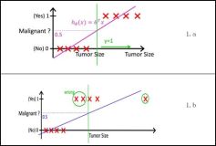
Logistic Regression,罗吉斯回归

We use the logistic regression equation to predict the probability of a dependent variable taking the dichotomy values 0 or 1. Suppose x₁, x₂, ..., x_p (p > 1) are the independent variables, α and β_k (k = 1, 2, ..., p) are the parameters, and E(y) is the expected value of the dependent variable y, then the logistic regression equation is:

For example, in the built-in data set mtcars, the data column am represents the transmission type of the automobile model (0 = automatic, 1 = manual). With the logistic regression equation, we can model the probability of a manual transmission in a vehicle based on its engine horsepower and weight data.

非线性回归, 世间事务的关系不可能都是线性的, 所以要来研究非线性回归

Estimated Logistic Regression Equation

Using the generalized linear model, an estimated logistic regression equation can be formulated as below. The coefficients a and b_k (k = 1, 2, ..., p) are determined according to a maximum likelihood approach, and it allows us to estimate the probability of the dependent variable y taking on the value 1 for given values of x_k (k = 1, 2, ..., p).

Problem

By use of the logistic regression equation of vehicle transmission in the data set mtcars, estimate the probability of a vehicle being fitted with a manual transmission if it has a 120hp engine and weights 2800 lbs.

Solution

We apply the function glm to a formula that describes the transmission type (am) by the horsepower (hp) and weight (wt). This creates a generalized linear model (GLM) in the binomial family.

> am.glm = glm(formula=am ~ hp + wt,  
+              data=mtcars,  
+              family=binomial)

We then wrap the test parameters inside a data frame newdata.

> newdata = data.frame(hp=120, wt=2.8)

Now we apply the function predict to the generalized linear model am.glm along with newdata. We will have to select response prediction type in order to obtain the predicted probability.

> predict(am.glm, newdata, type="response")  
      1  
0.64181

Significance Test for Logistic Regression

We can decide whether there is any significant relationship between the dependent variable y and the independent variables x_k (k = 1, 2, ..., p) in the logistic regression equation. In particular, if any of the null hypothesis that β_k = 0 (k = 1, 2, ..., p) is valid, then x_k is statistically insignificant in the logistic regression model.

本文章摘自博客园，原文发布日期：2012-03-02