谁更胜一筹?--随机搜索 V.S. 网格搜索
在进行超参数优化工作时,我不断思考该使用随机搜索还是网格搜索呢?这时候,一个同事给我介绍了一篇由Bergstra和Bengio编写的随机搜索超参数优化论文(链接),文中认为在进行参数优化时随机搜索比网格搜索更有效。
我想通过测试来得到自己的答案,我的实验设置如下。给定空间为(1024,1024)的超参数空间,可由相同形状的矩阵表示。我们为寻找最佳超参数设置的预算是25个实验。因此,这将允许我们进行网格搜索,其中我们设置每个超参数有5个值的组合,或者在该空间中的25个随机搜索。此外,我设置了一个“批量”版本的随机搜索,执行5批次每批次5次随机搜索,优化调整每次批次后的搜索。生成多个这样的随机超参数空间后,计算两种随机搜索优于网格搜索的次数。
生成空间
这一步是生成随机2D超参数空间,例如某种地形。 我使用了Hill地形算法(链接)。 它是一个简单而优雅的算法。 代码如下:
| 1 2 3 4 5 6 7 8 9 10 11 12 13 14 15 16 17 18 19 20 21 22 23 24 25 26 27 28 29 30 31 32 33 34 35 36 37 38 |
from __future__ import division, print_function import numpy as np import matplotlib.pyplot as plt import matplotlib.cm as cm import operator %matplotlib inline
SIZE = 1024 NUM_ITERATIONS = 200
terrain = np.zeros((SIZE, SIZE), dtype="float") mod_iter = NUM_ITERATIONS // 10 for iter in range(NUM_ITERATIONS): if iter % mod_iter == 0: print("iteration: {:d}".format(iter)) r = int(np.random.uniform(0, 0.2 * SIZE)) xc, yc = np.random.randint(0, SIZE - 1, 2) z = 0 xmin, xmax = int(max(xc - r, 0)), int(min(xc + r, SIZE)) ymin, ymax = int(max(yc - r, 0)), int(min(yc + r, SIZE)) for x in range(xmin, xmax): for y in range(ymin, ymax): z = (r ** 2) - ((x - xc) ** 2 + (y - yc) ** 2) if z > 0: terrain[x, y] += z print("total iterations: {:d}".format(iter)) # 标准化单元高度 zmin = np.min(terrain) terrain -= zmin zmax = np.max(terrain) terrain /= zmax # 通过z值平滑地形 terrain = np.power(terrain, 2) # 乘以255以使地形以灰度表示 terrain = terrain * 255 terrain = terrain.astype("uint8") |
从上面代码生成的一个可能的地形如下所示。 我还为它生成了一个等高线图。
| 1 2 3 4 5 6 7 8 9 |
plt.title("terrain") image = plt.imshow(terrain, cmap="gray") plt.ylim(max(plt.ylim()), min(plt.ylim())) plt.colorbar(image, shrink=0.8)
plt.title("contours") contour = plt.contour(terrain, linewidths=2) plt.ylim(max(plt.ylim()), min(plt.ylim())) plt.colorbar(contour, shrink=0.8, extend='both') |

网格搜索
如您所见,地形只是一个形状矩阵(1024,1024)。 由于我们的预算是25个实验,我们将在这个地形上进行一次5x5的网格搜索。 意即在x和y轴上选择5个等距点,并读取这些(x,y)位置处的地形矩阵值。 执行此操作的代码如下所示。 在轮廓图上的点的最佳值以蓝色标示。
|
1 2 3 4 5 6 7 8 9 10 11 12 13 14 15 16 17 18 19 20 21 |
# 执行 (5x5)网格搜索 results = [] for x in np.linspace(0, SIZE-1, 5): for y in np.linspace(0, SIZE-1, 5): xi, yi = int(x), int(y) results.append([xi, yi, terrain[xi, yi]])
best_xyz = [r for r in sorted(results, key=operator.itemgetter(2))][0] grid_best = best_xyz[2] print(best_xyz)
xvals = [r[0] for r in results] yvals = [r[1] for r in results]
plt.title("grid search") contour = plt.contour(terrain, linewidths=2) plt.ylim(max(plt.ylim()), min(plt.ylim())) plt.scatter(xvals, yvals, color="b", marker="o") plt.scatter([best_xyz[0]], [best_xyz[1]], color='b', s=200, facecolors='none', edgecolors='b') plt.ylim(max(plt.ylim()), min(plt.ylim())) plt.colorbar(contour) |

网格搜索中最优点坐标为(767,767),值为109。
随机搜索
接下来进行实验的是纯随机搜索。由于实验预设为25个,所以这里仅随机生成x值和y值,然后在这些点中搜索地形矩阵值。
| 1 2 3 4 5 6 7 8 9 10 11 12 13 14 15 16 17 18 19 20 21 |
# 进行随机搜索 results = [] xvals, yvals, zvals = [], [], [] for i in range(25): x = np.random.randint(0, SIZE, 1)[0] y = np.random.randint(0, SIZE, 1)[0] results.append((x, y, terrain[x, y]))
best_xyz = sorted(results, key=operator.itemgetter(2))[0] rand_best = best_xyz[2] print(best_xyz)
xvals = [r[0] for r in results] yvals = [r[1] for r in results]
plt.title("random search") contour = plt.contour(terrain, linewidths=2) plt.ylim(max(plt.ylim()), min(plt.ylim())) plt.scatter(xvals, yvals, color="b", marker="o") plt.scatter([best_xyz[0]], [best_xyz[1]], color='b', s=200, facecolors='none', edgecolors='b') plt.colorbar(contour) |

在该测试中,随机搜索做得更好一些,找到坐标为(663,618)值为103的点。
批量随机搜索
在这种方法中,我决定将我的25个实验预算分成5批,每批5个实验。 查找(x,y)值在每个批次内是随机的。 同时,在每个批次结束时,优胜者会被挑出来进行特殊处理。 采用对象不是在空间中任何地方生成的点,而是在这些点周围绘制一个窗口,并且仅从这些空间进行采样。 在每次迭代时,窗口会进行几何收缩。我试图寻找到目前为止找到的最优点的邻域中的点,希望这个搜索将产生更多的最优点。 同时,我保留剩余的实验探索空间,希望我可能找到另一个最佳点。 其代码如下所示:
| 1 2 3 4 5 6 7 8 9 10 11 12 13 14 15 16 17 18 19 20 21 22 23 24 25 26 27 28 29 30 31 32 33 34 35 36 37 38 39 40 41 42 43 44 45 46 47 48 49 50 51 52 53 54 55 56 57 58 59 60 61 62 |
def cooling_schedule(n, k): """ 每次运行时减少窗口的大小 n – 批次数目 k – 当前批次的索引号 返回 乘数(0..1) 的大小 """ return (n - k) / n
results, winners = [], [] for bid in range(5): print("Batch #: {:d}".format(bid), end="")
# 计算窗口大小 window_size = int(0.25 * cooling_schedule(5, bid) * SIZE)
# 计算出优胜者并把其值加入结果中 # 只保持最优的两点 for x, y, _, _ in winners: if x < SIZE // 2: # 中左区 xleft = max(x - window_size // 2, 0) xright = xleft + window_size else: # 中右区 xright = min(x + window_size // 2, SIZE) xleft = xright - window_size if y < SIZE // 2: # 下半区 ybot = max(y - window_size // 2, 0) ytop = ybot + window_size else: # 上半区 ytop = min(y + window_size // 2, 0) ybot = ytop - window_size xnew = np.random.randint(xleft, xright, 1)[0] ynew = np.random.randint(ybot, ytop, 1)[0] znew = terrain[xnew, ynew] results.append((xnew, ynew, znew, bid))
# 添加剩余随机点 for i in range(5 - len(winners)): x = np.random.randint(0, SIZE, 1)[0] y = np.random.randint(0, SIZE, 1)[0] z = terrain[x, y] results.append((x, y, z, 2))
# 找出最优两点 winners = sorted(results, key=operator.itemgetter(2))[0:2] print(" best: ", winners[0])
best_xyz = sorted(results, key=operator.itemgetter(2))[0] print(best_xyz)
xvals = [r[0] for r in results] yvals = [r[1] for r in results]
plt.title("batched random search") contour = plt.contour(terrain, linewidths=2) plt.ylim(max(plt.ylim()), min(plt.ylim())) plt.scatter(xvals, yvals, color="b", marker="o") plt.scatter([best_xyz[0]], [best_xyz[1]], color='b', s=200, facecolors='none', edgecolors='b') plt.colorbar(contour) |
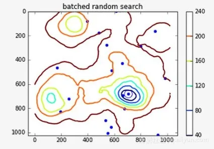
结束时此空间中的全局最小点坐标(707,682),值为20。
显然,并不是所有的运行都是如此顺利的,也很有可能从上述任何方法发现的点只是一个局部最小值。 此外,没有理由假定网格搜索可能不优于随机搜索,因为随机地形可能在其中一个均匀布置的点下面具有其全局最小点,并且随机搜索可能错过该点。
为了检查这个假设,我对1000个随机地形批量运行上面的代码。 对于每个地形,我为3种方法中的每一种运行25个实验,并为每个方法找到最低(最优)点。我这样做了两次,以确保结果的客观性。代码如下:
| 1 2 3 4 5 6 7 8 9 10 11 12 13 14 15 16 17 18 19 20 21 22 23 24 25 26 |
TERRAIN_SIZE = 1024 NUM_HILLS = 200
NUM_TRIALS = 1000 NUM_SEARCHES_PER_DIM = 5 NUM_WINNERS = 2
nbr_random_wins = 0 nbr_brand_wins = 0 for i in range(NUM_TRIALS): terrain = build_terrain(TERRAIN_SIZE, NUM_HILLS) grid_result = best_grid_search(TERRAIN_SIZE, NUM_SEARCHES_PER_DIM) random_result = best_random_search(TERRAIN_SIZE, NUM_SEARCHES_PER_DIM**2) batch_result = best_batch_random_search(TERRAIN_SIZE, NUM_SEARCHES_PER_DIM, NUM_SEARCHES_PER_DIM, NUM_WINNERS) print(grid_result, random_result, batch_result) if random_result < grid_result: nbr_random_wins += 1 if batch_result < grid_result: nbr_brand_wins += 1
print("# times random search wins: {:d}".format(nbr_random_wins)) print("# times batch random search wins: {:d}".format(nbr_brand_wins)) |
执行结果如下:
| 1 2 3 4 5 6 7 8 9 |
Run-1 ------ #-times random search wins: 619 ‘随机搜索优胜次数 #-times batch random search wins: 638 ‘随机批量搜索优胜次数
Run-2 ------ #-times random search wins: 640 ‘随机搜索优胜次数 #-times batch random search wins: 621随机批量搜索优胜次数 |
结果表明随机搜索似乎比网格搜索稍好(因为第一个数字超过500)。 此外,批量版本不一定更好,因为纯随机搜索在第二次运行有更好的结果。
以上是我实验的结果。在这个过程中,我学习了一个有趣的算法来生成地形,也为自己解除了困惑。如果你想亲自尝试,不妨阅读本文核心笔记(链接)以及批处理运行Python版本代码(链接)。
数十款阿里云产品限时折扣中,赶紧点击领劵开始云上实践吧!
作者简介:
Sujit Pal是一名程序员,在Healline Networks担任技术管理。喜好研究编程语言Java和Python,喜欢从多角度研究和解决问题。
本文由北邮@爱可可-爱生活 老师推荐,阿里云云栖社区组织翻译。
文章原标题《Random vs Grid Search: Which is Better?》,作者:Sujit Pal ,译者:伍昆