摘要:
2018 年“双 11”的交易额又达到了一个历史新高度 2135 亿。相比十年前,我们的交易额增长了 360 多倍,而交易峰值增长了 1200 多倍。相对应的,系统数呈现爆发式增长。系统在支撑“双 11”过程中的复杂度和难度呈现指数级形式上升趋势。
作为阿里巴巴全集团范围的容器调度系统,Sigma 在“双11”期间成功支撑了全集团所有容器(交易线中间件、数据库、广告等 20 多个业务)的调配,是阿⾥巴巴运维系统重要的底层基础设施。Sigma 已经是阿里全网所有机房在线服务管控的核心角色,管控的宿主机资源达到百万级,重要程度不言而喻,其算法的优劣程度影响了集团整体的业务稳定性,资源利用率。
当用戶向调度系统申请容器所需的计算资源(如 CPU 、 内存、磁盘)时,调度器负责挑选出满足各项规格要求的物理机来部署这些容器。在相同的资源需求下,调度策略的优劣决定着集群计算资源利用的水平。本文将简要介绍群体增强学习算法在调度策略优化中的应用。
作者:
王孟昌 达摩院机器智能技术算法专家
韩堂 阿里巴巴集团技术专家
1.计算资源调度及在线策略
当用户向 Sigma 申请容器所需的计算资源(如 CPU、Memory、磁盘等)时,调度器负责挑选出满足各项规格要求的物理机来部署这些容器。通常,满足各项要求的物理机并非唯一,且水位各不相同,不同的分配方式最终得到的分配率存在差异,因此,调度器的一项核心任务就是按照某一策略从众多候选机器中挑出最合适的物理机。
在文献中,计算资源调度一般被表述为矢量装箱问题(vector bin packing problem),如果各应用的容器数量事先已知(如大促场景),调度器可一次性为所有容器生成优化的排布方案,此时问题可以表述为整数规划,可使用通用求解器或专门开发的算法来求解;如果各应用的请求陆续到达 Sigma (如日常场景),调度器需要在每次请求到达时即时(在线)生成部署决策,此时问题可表述为马尔可夫决策过程 (Markov Decision Process, MDP),原则上可以通过值迭代或策略迭代求得最优策略。
最常用的调度策略包括 First-Fit (FF) 和 Best-Fit (BF)。如果使用 First-Fit算法,调度器会将容器部署到遍历中碰到的第一个满足所有要求的物理机上;而Best-Fit算法则会在满足要求的物理机中挑选分配水位最高的机器来部署容器。对于经典的 bin packing 问题(即一维矢量装箱问题),First-Fit 和 Best-Fit 的近似比均为1.7,即二者都可保证所使用的机器数不超出最优方案的170%;对于2维及以上的矢量装箱问题,理论上不存在有着明确近似比保证的多项式算法。当物理机的某个资源维度明显为瓶颈而导致其它资源维度普遍有剩余时,其有效维度可视为1,使用 First-Fit 或 Best-Fit 一般可以取得不错的分配率;而一旦瓶颈并未集中体现在同一维度,两种策略的效果就要大打问号了。
除了资源维度上的要求,实际调度中还有容灾和干扰隔离上的考虑:比如同一应用的容器不允许全部部署到同一台物理机上,很多应用甚至每台机器上只允许有一个实例;某些应用之间还存在互斥关系(如资源争抢),严重影响应用的性能,因此也不允许它们被部署到同一物理机上。这些限制条件的引入,使得常用策略越发水土不服了。通过人肉反复试错,勉强扛住了多次大促建站的压力。然而,随着各业务的扩张,线上容器的规模越来越大,资源变得越来越紧张,人肉调参的效率渐渐力不从心。
为了把调度同学从调参中解放出来,让有限的资源扛住更大的压力,达摩院机器智能技术实验室(M.I.T.)的决策智能算法团队和Sigma调度团队展开了紧密合作,对在线调度策略问题进行了研究,并开发了基于群体增强学习(SwarmRL)的算法。
2.在线调度模型
记当前待部署容器的规格为向量 p∈P,为其分配资源时集群状态为向量 s∈S , 候选物理机的集合为 A⊆A,策略可表示为函数 π:S×P→A(π∈Π)。当按策略 π 选择物理机 a=π(s,p)来部署该容器时,该选择的即时成本为 r(a),集群的新状态 s′ 由状态量 s 、p 以及动作 a 共同决定,记为 s′=L(s,p,a) ;记后续到达的容器规格 p′, 对于在线调度,p′ 为随机量。引入折扣系数 γ∈[0,1],系统的 Bellman 方程为:

最优调度策略可表示为:

理论上,通过随机梯度下降,我们可以在策略空间 Π 中搜索较优的策略,但相要更进一步的优化,甚至得到全局最优策略,则需要借助其它方法,特别是当最优策略可能是 multi-modal 形式。
3.群体增强学习 SwarmRL
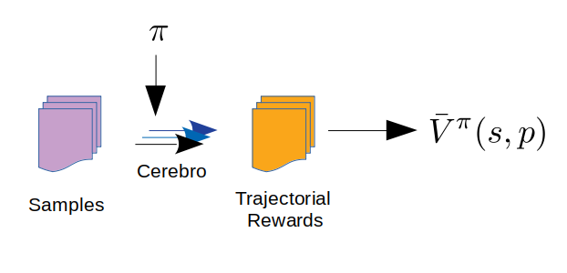
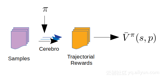
为防止策略的优化陷入较差的局部最优解,同时拥有较快的收敛速度,我们基于群体增加学习的框架来设计算法。与传统的增强学习方法相比,算法使用多个 agent 来探索问题的策略空间,且多个 agent 之间存在互相学习机制,这使得算法有了跳出局部陷阱的能力。为获取各状态值(V^π^)的估计,一个准确的 Sigma 模拟器必不可少,团队内部同学基于 Sigma 的调度器开发了“完全保真”的模拟器 Cerebro 。
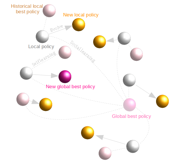
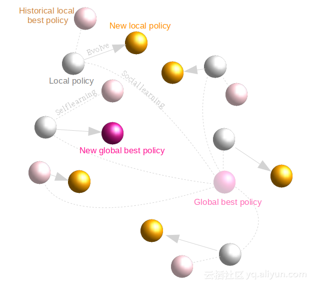
算法首先随机初始化一群 agent 的策略,针对每个策略,通过模拟器获取相应的的状态值估计,记录当前全局最佳策略。在后续的每次迭代中,各个 agent 不断更新自身的局部最佳策略,并参照局部最佳策略与群体当前全局最佳策略,对 agent 自身的当前策略进行更新,再进行模拟,获取新策略的状态值估计,更新全局最佳策略。如此循环,直到满足收敛条件。
在各个 agent 状态值的估计中,样本(多个随机抽取的集群快照和扩容请求序列)和各 agent 的当前策略被输入模拟器 Cerebro,追踪模拟时集群状态的轨迹,即可得到该轨迹的总成本;基于多个样本的轨迹总成本求平均,即得到相应策略下的状态估计值。
在 SwarmRL 中,策略的演进方向与步长用“速度” (v) 来表示,速度的变化涉及局部最佳策略 (πL) 和群体全局最佳策略 (πG ) 与 agent 当前策略 (π) 的差异,并受策略惯性因子 w、本地学习因子C~1~(self-learning)、群体学习因子 C~2~ (social-learning) 等参数的调控:

其中 ξ1,ξ2∈[0,1] 为随机量,Φ为可行性保持映射,用于将逸出可行域的 agent 重新“拉回”可行域。在迭代中,局部最佳策略 (πL) 和群体全局最佳策略 (πG ) 不断更新:
4.算法应用
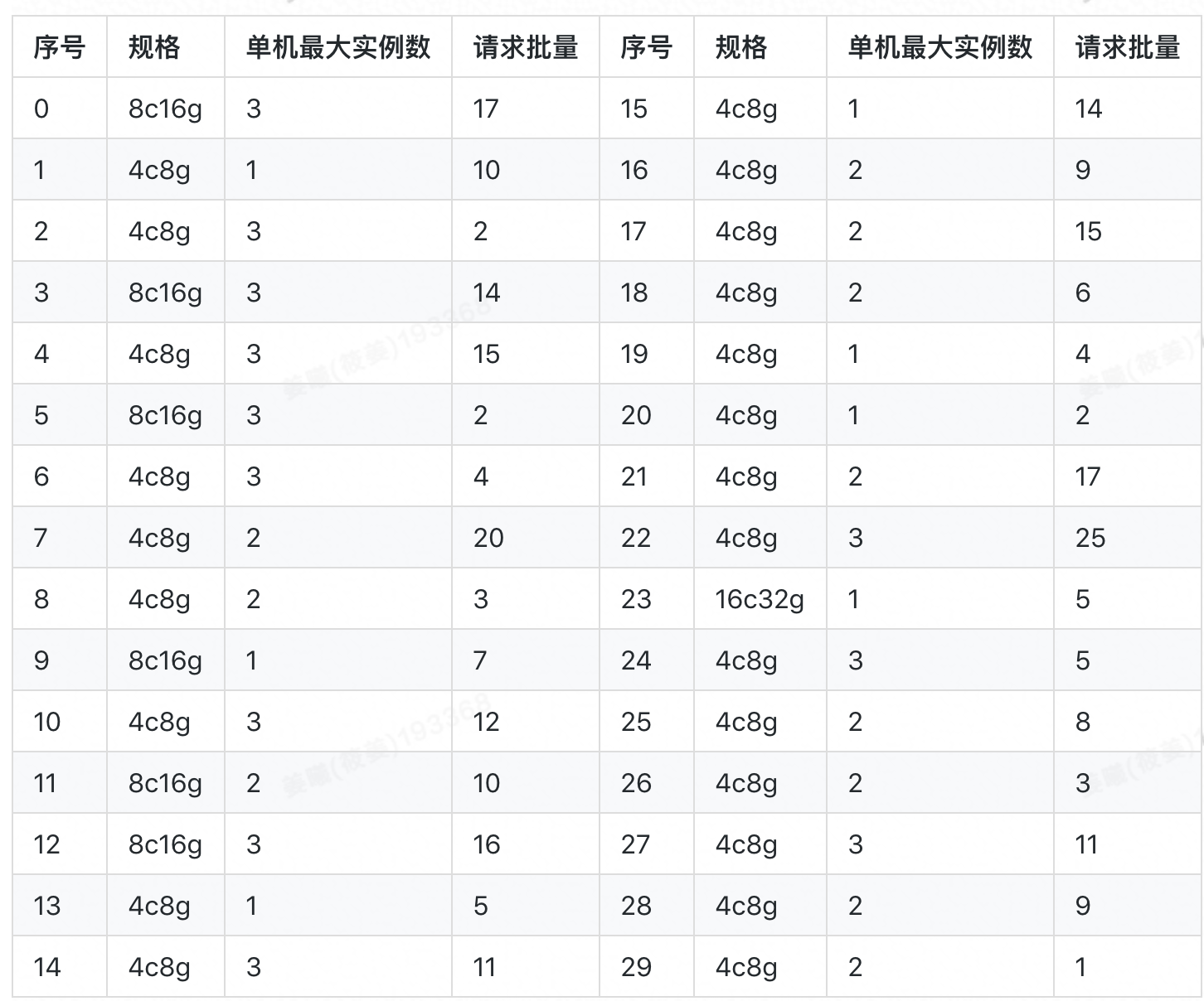
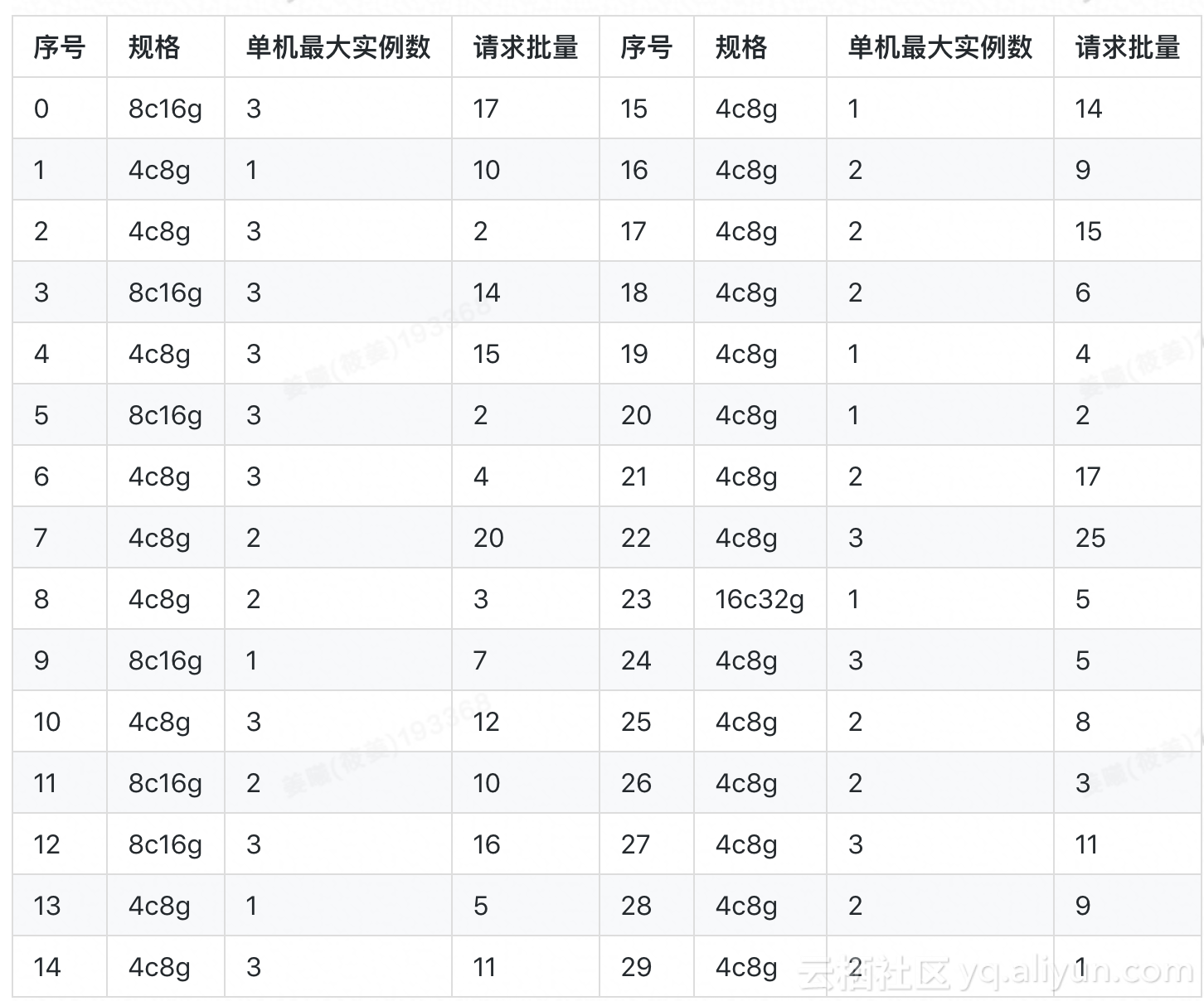
下面我们先用一个随机生成的小算例来对比一下算法的效果。算例中涉及 30 个应用(见下表),其容器规格主要为 4c8g 与 8c16g,所用宿主机的规格均为 96c512g。
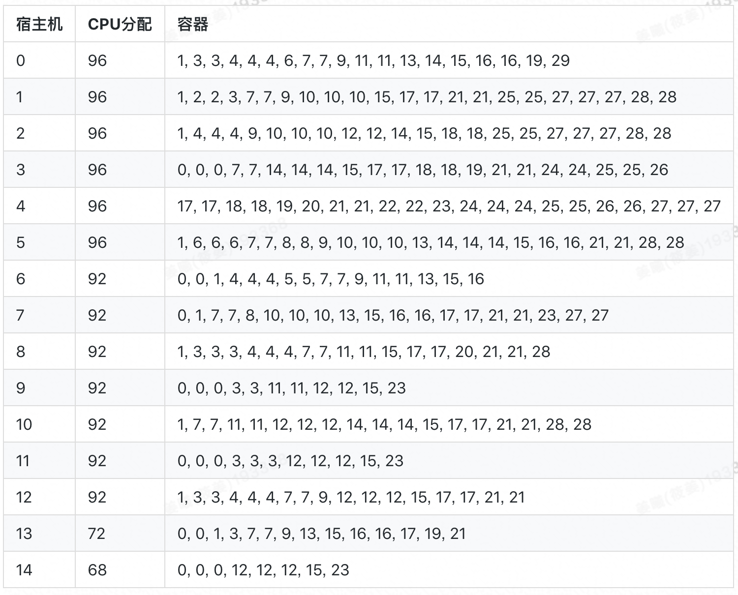
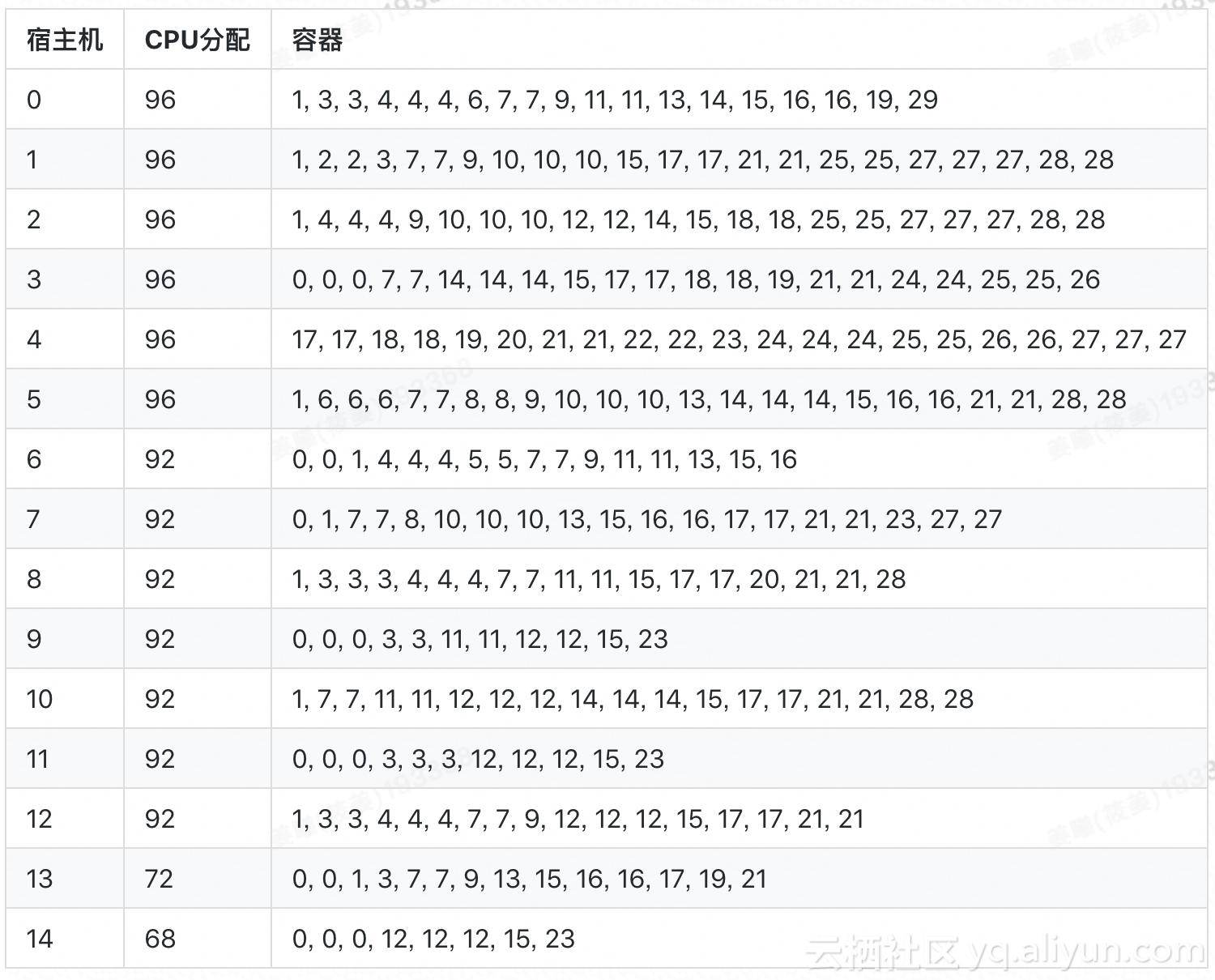
若在调度时,请求的顺序和数量均为已知(“上帝视角”),即进行事后排布,使用整数规划求得的最优解对应的分配率为 94.44 % (这也是所有调度策略在该算例上所得分配率的上界),共启用 15 台宿主机,具体排布方案为:
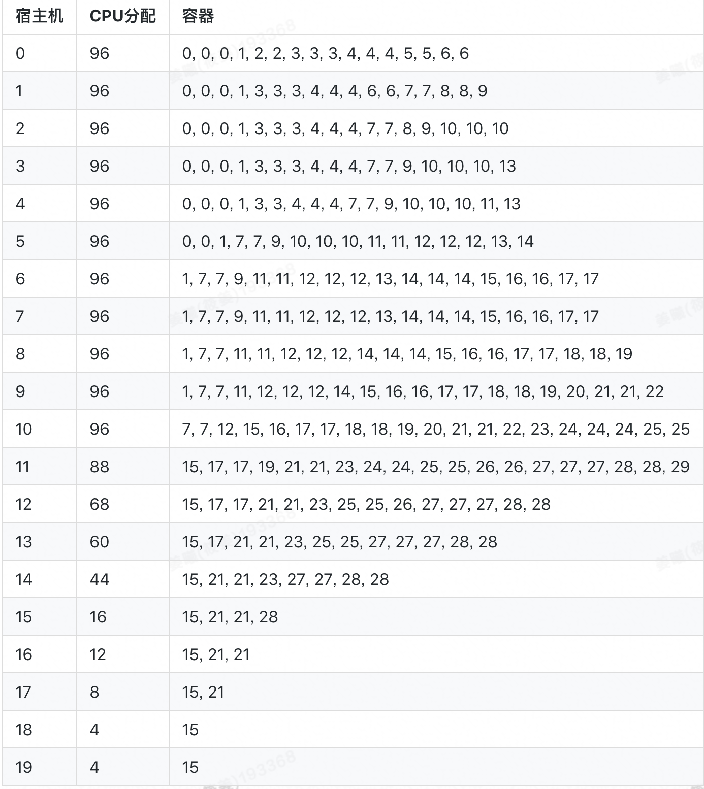
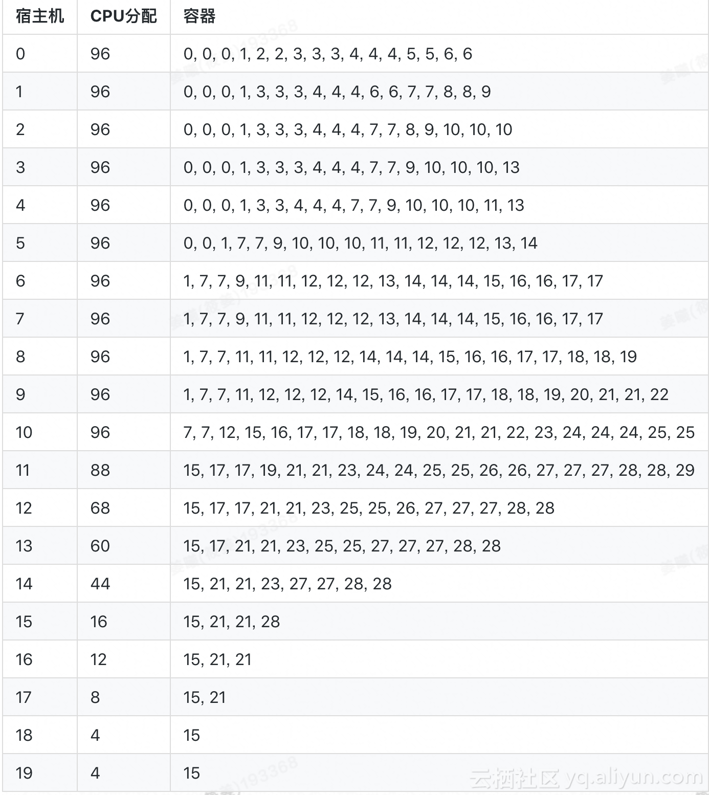
现实场景中,每个请求所处顺序和容器数量仅在其到达 Sigma 时才揭晓,若采用 Best-Fit 进行动态调度,所得分配率为 70.83%,共启用 20 台宿主机,具体排布如下:
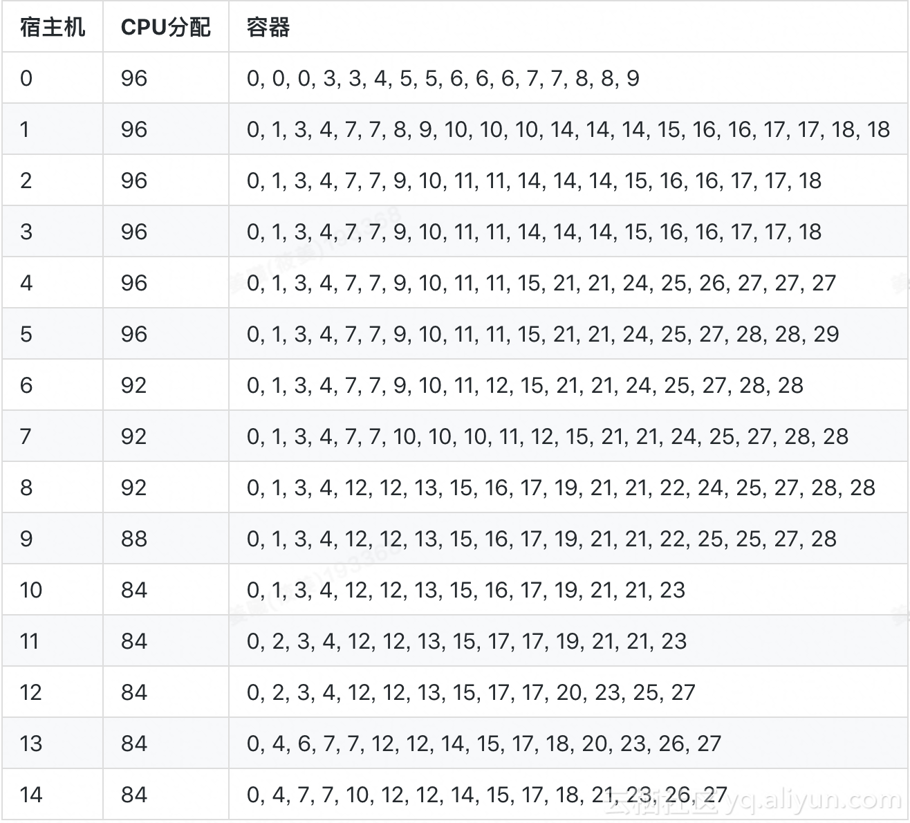
若采用 SwarmRL 学习所得策略进行动态分配,分配率为 94.44%,共启用 15 台宿主机,最终容器排布如下:
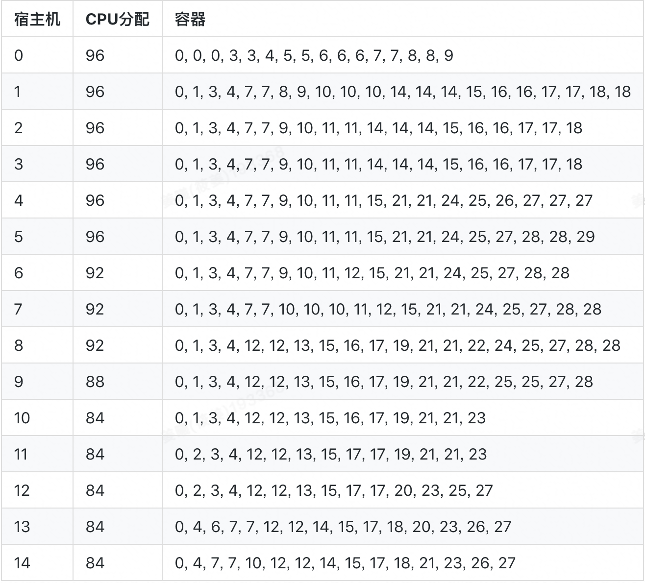
在该算例中,SwarmRL 学习所得策略的表现(94.44%)与“上帝视角”下最优排布的表现(上界)一致,明显优于 Best-Fit 的表现(70.83%),改进幅度达 23.61%.
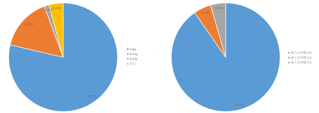
我们再随机生成规模较大的请求数据:共计 3K 个请求,5K 个容器,其规格分布如下图,
由于该场景下整数规划模型的变量规模太大,已经无法在短时间内直接求取“上帝视角”的最优解。对比 Best-Fit (以及人肉策略),算法所得新策略的效果如下:

相对于 Best-Fit,新策略节约宿主机 13 台(4.48%),分配率提升 4.30%;相对于人肉策略,新策略节约 7 台(2.46%)宿主机,分配率改进 2.36%.
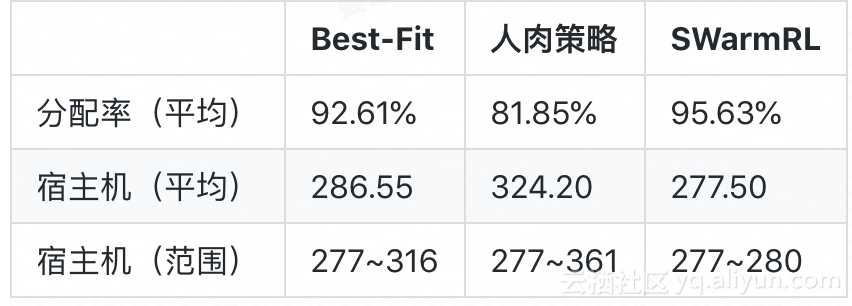
考虑到实际场景中应用请求到达顺序的随机性,我们随机打乱请求生成多个不同的请求顺序,再分别应用三个策略按不同的请求顺序进行动态分配:
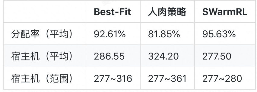
Best-Fit 在不同请求顺序下宿主机数量的极差为 39 台,相对人肉策略的 84 台而言,表现相对稳定,其波动幅度约为人肉策略的一半;人肉策略的平均分配率低至 81.85%,对比原顺序下的 93.44%,可见人肉策略的性能并不稳定,表现出较剧烈的波动。而学习所得新策略的表现则相当稳定,其宿主机数量的极差仅为 3 台,波动幅度约为人肉策略的 30 分之一;新策略的分配率平均比人肉策略的分配率高 13.78%,比 Best-Fit 的高 3.02%.
5.总结与展望
从提升分配率、节省资源的角度来看,SwarmRL 算法可以产生出优于常用(以及人肉)的策略,并且有着较为稳定的表现。算法部署到线上环境后,公共资源池的分配率峰值与之前相比有了明显的提升。
随着 CPU share 和混部的铺开,除分配率外,新的场景将涉及更多目标,比如打散、负载均衡等,这些目标甚至还有互相矛盾的地方,而 SwarmRL 的运行机制天然适合具有多个目标的策略优化问题,可以十分方便地在策略空间中构造 Pareto Front,因而,后续我们将继续研究新场景下的在线调度策略问题,充分挖掘 SwarmRL 的潜力,进一步提升 Sigma 的调度能力。
参考文献
- David Simchi-Levi, Xin Chen and Julien Bramel (2014). The Logic of Logistics: Theory, Algorithms, and Applications for Logistics Management (3rd ed). Springer
- Richard S. Sutton and Andrew G. Barto (2017). Reinforcement Learning: An Introduction. The MIT Press
- Hitoshi Iima, Yasuaki Kuroe and Kazuo Emoto (2011). Swarm reinforcement learning methods for problems with continuous state-action space, IEEE ICSMC
- Yossi Azar, Ilan R. Cohen, Amos Fiat and Alan Roytman (2016). Packing small vectors. SODA'16
- Yossi Azar, Ilan R. Cohen, Seny Kamara and Bruce Shepherd (2013). Tight bounds for online vector bin packing. STOC‘13
英文版(感谢谷歌:Yaxiong Zhao 翻译)
Beating Best-Fit hands down: How Alibaba optimizes Sigma’s online scheduling policy to save hundreds of millions
Abstract:
In 2018’s Singles Day (Double 11), Alibaba once again set a new record GMV totaled 213.5 billion yuan. Compared to a decade ago, our GMV has increased by more than 360 times, and the peak transaction rate has increased by more than 1,200 times. To support such explosive growth, the number of systems have increased exponentially; their complexity and the difficulty of working with these systems have been and are still increasing exponentially.
Sigma is Alibaba's foundational container orchestration system supporting all Alibaba Group subsidiaries, and a critical component in Alibaba’s production infrastructure. Sigma schedules and manages all containers of the entire Alibaba Group (transaction line middleware, Database, ADs, etc.) during the Singles Day. Sigma is the core for managing all Alibaba’s online service in all data centers, controls millions of physical servers. Its algorithms determine the stability of Alibaba’s business operations and the utilization of hardware resources. Its importance is self-evident.
When a user requesting resources (such as CPU, RAM, disk) from Sigma to run containers, it is the Sigma scheduler that selects the physical servers. For the same resource requirements, the quality of the scheduling policy determines the resource utilization. This paper introduces the application of swarm reinforcement learning in optimizing the scheduling policy.
Author:
**Wang Mengchang: Dharma Institute Machine Intelligent Technology, Algorithm Expert
Han Tang: Alibaba Group, Technical Expert**
1. Computing resource scheduling and online scheduling policy
When a user requesting resources (such as CPU, RAM, disk) from Sigma to run containers, it is the Sigma scheduler that selects the physical servers. There are often more servers that meet the requirements than the requested amount. The current utilizations on these machines vary. The resulting utilizations of different scheduling policies vary as well. Therefore, one of the core functionalities of the Sigma scheduler is to select the most suitable physical server from a number of candidates according to a certain policy.
In the literature, computing resource scheduling is generally modeled as a vector bin packing problem. If the number of containers and their requirements are known in advance (such as a large promotion event), the scheduler can generate the optimal placement for all containers at once. In this case, the problem can be modeled as an integer programming problem, which can be solved using a general-purpose solver or a specially developed algorithm. If the scheduling requests to Sigma comes continuously (such as normal daily operation), the scheduler must instantaneously compute the placement for each request (online decision making). In this case, the problem can be modeled as a Markov Decision Process (MDP). In principle, the optimal scheduling policy can be obtained through value iteration or policy iteration.
The most common scheduling policies include First-Fit (FF) and Best-Fit (BF). In First-Fit, the first physical server that meet all the requirements of a container is selected; in Best-Fit, the machine with the highest utilization is selected. For the classic bin packing problem (ie, one-dimensional vector packing problem), the approximate ratio of First-Fit and Best-Fit is both 1.7, that is, both can ensure that the number of machines required does not exceed 170% of the optimal solution. For the vector packing problem of 2D and above, there is no polynomial algorithm with a fixed approximation ratio. When there is only one resource dimension that is the bottleneck in the fleet and other resource dimensions are generally abundant, the effective dimension can be regarded as 1. Using First-Fit or Best-Fit can usually achieve a good utilization. In other situations, the quality of the these two policies will be a big question mark.
In addition to optimizing the resource utilization, scheduling policies also consider other restrictions like fault-tolerance and isolation. For example, all of the containers of an application are not allowed to be deployed on the same physical machine, and many applications only allow at most one instance per physical machine. There can also be conflicts between applications (such as resource contentions), which seriously affect the performance of the applications when they are running on the same machine; and therefore they are not allowed to be run on the same machine. These restrictions further make the vanila policy inappropriate in practice. Sigma barely withstands the pressure of several large promotion events, through repeated trial and error of manual parameter tuning. However, Alibaba’s aggressive business expansion results into rapid-growing in the scale of the container deployment, the resource contention have become more and more severe; and the velocity of manual parameter-tuning are gradually failing behind.
In order to free our colleagues working on Sigma scheduling from the tedious manual parameter tuning, and let the limited resources be utilized more efficiently, the Machine Intelligence Lab of DAMO Academy and the Sigma team have started a collaboration. We studied the optimal policy for online scheduling, and developed an algorithm based on swarm reinforcement learning (SwarmRL).
2. Online scheduling model
The current specification of the container to be deployed is a vector p∈P. When the resource is allocated, the cluster state is vector s∈S, the set of candidate physical machines is A⊆A, and the policy can be expressed as function π: S×P→A(π ∈Π). When the container is deployed by selecting the physical machine a=π(s,p) according to the policy π, the immediate cost of the selection is r(a), and the new state of the cluster s' is determined by the previous state s, container specifications p, and the action a. It is denoted as s'=L(s,p,a); let p’ be the container specification that arrives later, for online scheduling, p' is a random quantity. Introducing the discount coefficient γ∈[0,1], the Bellman equation of the system is:

The optimal scheduling policy can be expressed as:

In theory, we can use stochastic gradient descent to find optimized policies in the policy space. However, if we were to further optimize or even get the global optimal policy, we need to use other methods, especially when the optimal policy were Multi-modal.
3. Swarm Reinforcement Learning: SwarmRL
In order to avoid inferior local optimums and achieve fast convergence speed, we designed the algorithm based on Swarm Reinforcement Learning (SwarmRL). Compared with traditional reinforcement learning methods, SwarmRL employs multiple agents to explore the policy space of the optimization problem, and there are mutual learning mechanisms among multiple agents, which allows the learning process to jump out of local optimums. To accurately estimate each state value (V^π^), an high-fidelity Sigma simulator is critical. We developed an full-fidelity simulator called Cerebro, based on Sigma scheduler.
The algorithm first randomly initializes a group of agent policies. For each policy, the algorithm obtains the initial state value estimates from simulations and records the current global optimal policy. In each subsequent iteration, each agent continuously updates its local optimal policy, and the current effective policy in reference to the local optimal policy and the current global optimal policy of the group. The above process is repeated until the convergence condition is met.
To obtain the state estimate of a given policy for each agent, the sample (multiple randomly extracted snapshot of the cluster state and pending container requests sequence) and the agent’s current policy are fed to the simulator Cerebro, and the trajectory of the cluster state during the simulation is tracked to obtain the total cost of the trajectory. Averaging the total cost of the trajectories of multiple samples, the resultant average is the state estimate of the corresponding policy.
In SwarmRL, the direction and step size of the evolution of the policy are expressed as “speed” (v), which involves the difference between the local best policy (πL) and the group global best policy (πG) and the agent current policy (π). And regulated by parameters such as strategic inertia factor w, local learning factor C~1~(self-learning), group learning factor C~2~ (social-learning):

Where ξ1, ξ2∈[0,1] are random variables, and Φ is a feasibility-preserving map, which is used to “pull back” the agent that escapes the feasible domain back to the feasible domain. During iterations, the local optimal policy (πL) and the group global optimal policy (πG) are constantly updated:
4. Algorithm application
Let's first compare various algorithms in a small experiment with randomly generated inputs. The experiment involves 30 applications (see table below). The container specifications are mainly 4c8g (4 CPU and 8GB RAM) and 8c16g, and the specifications of the host used are 96c512g.
If at the time of scheduling, the order and spec of requests are known ("God perspective"), that is, an after-fact scheduling, the utilization of the optimal solution produced by integer programming is 94.44% (this is also the upper bound of the utilization of all scheduling policies). This solution requires a total of 15 machines. The actual placement is as follows:
In reality, the order and spec of each request are only revealed when they arrive at Sigma. The Best-Fit policy achieved a utilization of 70.83%, and a total of 20 hosts are required. The actual placement is as follows:
The policy learned from using SwarmRL achieved a utilization of 94.44%, and a total of 15 hosts are required. The actual placement is as follows:
In this experiment, the performance of the learned policy (94.44%) and that of from the "God perspective" (upper bound) is consistent, much better than the Best-Fit (70.83%), the improvement is 23.61%。
We then randomly generated larger data request: 3K requests, 5K containers. The requirements distribution is as follows: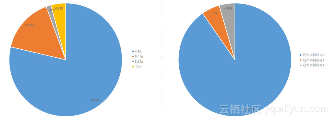
It is impossible to obtain the theoretical upper bound for this input, because the size of the Integer Programming is too large to solve in a reasonable small time. Here we omit the theoretical upper bound. Compared to Best-Fit (and manually tuned policy), the improvements of the learned policy is as follows:

Compared with Best-Fit, the learned policy saved 13 machines (4.48%), and the utilization is increased by 4.30%. Compared with the manually tuned policy, the learned policy saved 7 of machines (2.46%), and the utilization is increased by 2.36%.
Considering the random order of the application request arriving in real-world scenarios, we randomly reordered requests to generate multiple different request sequences, and then apply three policies to dynamically allocate machines:
Best-Fit has a small spread, 39 machines, in the number of required hosts from different input orders of the same set of requests. This is roughly half of that of the manually tuned policy, which is 84 machines. The average utilization of the manually-tuned policy is as low as 81.85%. Compared with 93.44% in the previous experiment, its performance is not stable and shows relatively severe fluctuations. The performance of the learned policy is quite stable. The spread of the number of required machines is only 3, and the fluctuation range is about one-third of that of the manually tuned policy. The utilization of the learned policy is 13.78% higher than that of the manually tuned policy, 3.02% higher than Best-Fit.
5. Summary and outlook
From the perspective of increasing the utilization and saving resources, SwarmRL can learn policies that perform better than common and manually-tuned policies; and the learned policies have a relatively stable performance. After the learned policy is deployed to production, the peak utilization of the public resource pool is significantly improved.
With the increasing adoption of CPU sharing and mixed online & offline workloads, new application scenarios will require optimizing for more objectives in addition to utilization, such as spread scheduling, load balancing, etc. These objectives are even contradictory in certain aspects. SwarmRL is naturally suitable for optimizing the policy for multiple objectives, as multiple objectives can be easily constructed as Pareto Front in the policy space. Therefore, we will continue to study the online scheduling policy problem in the new scenarios, fully realize the potential of SwarmRL, and further improve Sigma’s scheduling capability.
References
● David Simchi-Levi, Xin Chen and Julien Bramel (2014). The Logic of Logistics: Theory, Algorithms, and Applications for Logistics Management (3rd ed). Springer
● Richard S. Sutton and Andrew G. Barto (2017). Reinforcement Learning: An Introduction. The MIT Press
● Hitoshi Iima, Yasuaki Kuroe and Kazuo Emoto (2011). Swarm reinforcement learning methods for problems with continuous state-action space, IEEE ICSMC
● Yossi Azar, Ilan R. Cohen, Amos Fiat and Alan Roytman (2016). Packing small vectors. SODA'16
● Yossi Azar, Ilan R. Cohen, Seny Kamara and Bruce Shepherd (2013). Tight bounds for online vector bin packing. STOC‘13
