本课主要2个实践内容:


目前方向:图像拼接融合、图像识别 联系方式:jsxyhelu@foxmail.com
1、keras中数据集丰富,从数据集中提取更多特征(Data augmentation)
2、迁移学习(Tranform learning)
代码:https://github.com/jsxyhelu/DateSets
1、keras中数据集丰富,从数据集中提取更多特征(Data augmentation)
keras是比较现代化的DL工具,所以这方面的功能都是具备的。这里首先将相关知识进行整理,然后将例子进行实现,特别注重结果的展示。
具体内容包括:
- 旋转 | 反射变换(Rotation/reflection): 随机旋转图像一定角度; 改变图像内容的朝向;
- 翻转变换(flip): 沿着水平或者垂直方向翻转图像;
- 缩放变换(zoom): 按照一定的比例放大或者缩小图像;
- 平移变换(shift): 在图像平面上对图像以一定方式进行平移;
- 可以采用随机或人为定义的方式指定平移范围和平移步长, 沿水平或竖直方向进行平移. 改变图像内容的位置;
- 尺度变换(scale): 对图像按照指定的尺度因子, 进行放大或缩小; 或者参照SIFT特征提取思想, 利用指定的尺度因子对图像滤波构造尺度空间. 改变图像内容的大小或模糊程度;
- 对比度变换(contrast): 在图像的HSV颜色空间,改变饱和度S和V亮度分量,保持色调H不变. 对每个像素的S和V分量进行指数运算(指数因子在0.25到4之间), 增加光照变化;
- 噪声扰动(noise): 对图像的每个像素RGB进行随机扰动, 常用的噪声模式是椒盐噪声和高斯噪声;
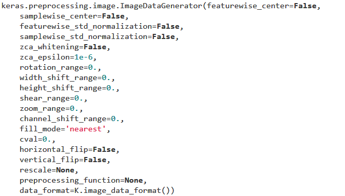
使用的函数为:
参数非常多,用以生成一个batch的图像数据,支持实时数据提升。训练时该函数会无限生成数据,直到达到规定的epoch次数为止;那么在训练的时候肯定是需要结合fit_generate来使用,正好是最近研究的。
主要方法:
a、
flow(self, X, y, batch_size=32, shuffle=True, seed=None, save_to_dir=None, save_prefix='', save_format='png')
将会返回一个生成器,这个生成器用来扩充数据,每次都会产生batch_size个样本。
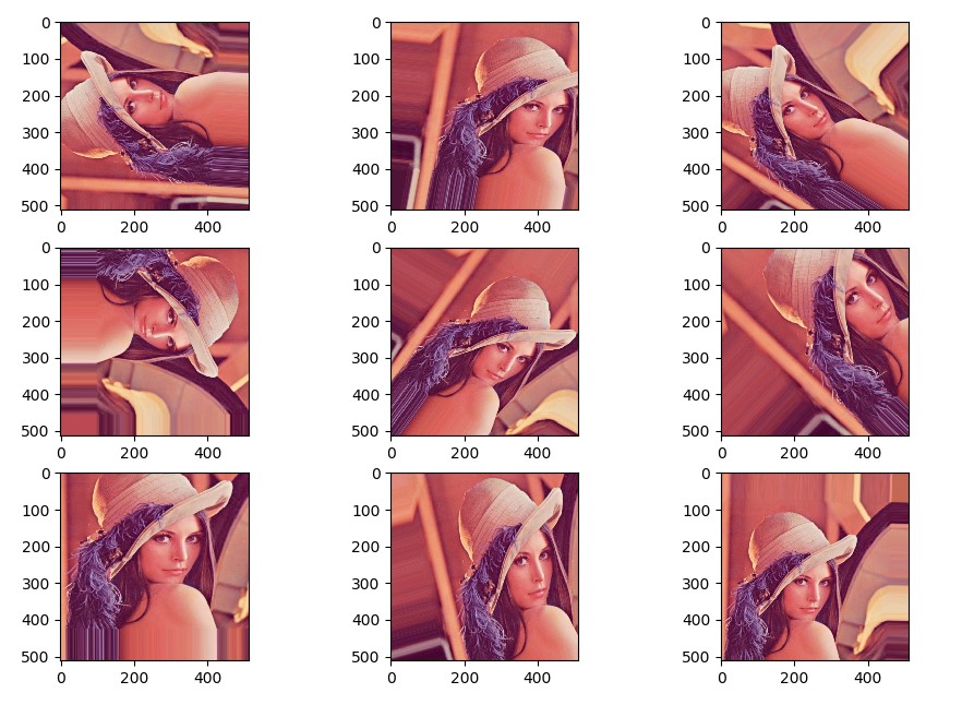
因为目前我们只导入了一张图片,因此每次生成的图片都是基于这张图片而产生的,可以看到结果,旋转、位移、放大缩小,统统都有。正如其名称,这个生成器可以一直生成下去。
b、flow_from_directory(directory):
以文件夹路径为参数,生成经过数据提升/归一化后的数据,在一个无限循环中无限产生batch数据
e.g
from keras.preprocessing.image
import ImageDataGenerator
from keras.preprocessing
import image
import matplotlib.pyplot
as plt
import numpy
as np
# 指定参数
# rotation_range 旋转
# width_shift_range 左右平移
# height_shift_range 上下平移
# zoom_range 随机放大或缩小
img_generator = ImageDataGenerator(
rotation_range =
90,
width_shift_range =
0.2,
height_shift_range =
0.2,
zoom_range =
0.3
)
# 导入并显示图片
img_path =
'e:/template/lena.jpg'
img = image.load_img(img_path)
plt.imshow(img)
plt.show()
# 将图片转为数组
x = image.img_to_array(img)
# 扩充一个维度
x = np.expand_dims(x,
axis=
0)
# 生成图片
gen = img_generator.flow(x,
batch_size=
1)
# 显示生成的图片
plt.figure()
for i
in
range(
3):
for j
in
range(
3):
x_batch =
next(gen)
idx = (
3*i) + j
plt.subplot(
3,
3, idx+
1)
plt.imshow(x_batch[
0]/
256)
x_batch.shape
plt.show()
代码中的绝对核心一句
gen = img_generator.flow(x,
batch_size=
1)
这样,gen相当于是img_generatror的一个生成器,下面直接使用next(gen)就可以不断生成。
e.g2验证DateAugment性能。
都说这个DateAugment好,但是不之际动手实践一下,总是不放心。
from keras.datasets
import cifar10
from keras.layers.core
import Dense, Flatten, Activation, Dropout
from keras.layers.convolutional
import Conv2D
from keras.layers.pooling
import MaxPooling2D
from keras.layers.normalization
import BatchNormalization
from keras.models
import Sequential
from keras.utils
import np_utils
from keras.preprocessing.image
import ImageDataGenerator
from keras.preprocessing
import image
import matplotlib.pyplot
as plt
import numpy
as np
from keras.utils
import generic_utils
(x_train, y_train),(x_test, y_test) = cifar10.load_data()
print(x_train.shape, y_train.shape, x_test.shape, y_test.shape)
def
preprocess_data(
x):
x /=
255
x -=
0.5
x *=
2
return x
# 预处理
x_train = x_train.astype(np.float32)
x_test = x_test.astype(np.float32)
x_train = preprocess_data(x_train)
x_test = preprocess_data(x_test)
# one-hot encoding
n_classes =
10
y_train = np_utils.to_categorical(y_train, n_classes)
y_test = np_utils.to_categorical(y_test, n_classes)
# 取 20% 的训练数据
x_train_part = x_train[:
10000]
y_train_part = y_train[:
10000]
print(x_train_part.shape, y_train_part.shape)
# 建立一个简单的卷积神经网络,序贯结构
def
build_model():
model = Sequential()
model.add(Conv2D(
64, (
3,
3),
input_shape=(
32,
32,
3)))
model.add(Activation(
'relu'))
model.add(BatchNormalization(
scale=
False,
center=
False))
model.add(Conv2D(
32, (
3,
3)))
model.add(Activation(
'relu'))
model.add(MaxPooling2D((
2,
2)))
model.add(Dropout(
0.2))
model.add(BatchNormalization(
scale=
False,
center=
False))
model.add(Flatten())
model.add(Dense(
256))
model.add(Activation(
'relu'))
model.add(Dropout(
0.2))
model.add(BatchNormalization())
model.add(Dense(n_classes))
model.add(Activation(
'softmax'))
return model
# 训练参数
batch_size =
128
#epochs = 20
epochs =
2
#cifar-10 20%数据,训练结果,绘图
model = build_model()
model.compile(
optimizer=
'adam',
loss=
'categorical_crossentropy',
metrics=[
'accuracy'])
model.fit(x_train_part, y_train_part,
epochs=epochs,
batch_size=batch_size,
verbose=
1,
validation_split=
0.1)
loss, acc = model.evaluate(x_test, y_test,
batch_size=
32)
print(
'Loss: ', loss)
print(
'Accuracy: ', acc)
#cifar-10 20%数据 + Data Augmentation.训练结果
# 设置生成参数
img_generator = ImageDataGenerator(
rotation_range =
20,
width_shift_range =
0.2,
height_shift_range =
0.2,
zoom_range =
0.2
)
model_2 = build_model()
model_2.compile(
optimizer=
'adam',
loss=
'categorical_crossentropy',
metrics=[
'accuracy'])
#采用文档中提示自动方法
img_generator.fit(x_train_part)
# fits the model_2 on batches with real-time data augmentation:
model_2.fit_generator(img_generator.flow(x_train_part, y_train_part,
batch_size=batch_size),
steps_per_epoch=
len(x_train_part),
epochs=epochs)
初步比较结果:
原始
Loss: 1.6311466661453247
Accuracy: 0.6169
调整
Epoch 1/20
2184/10000 [=====>........................] - ETA: 11:11 - loss: 1.0548 - acc: 0.6254
虽然没有走完,但是已经初见端倪。
2、迁移学习(Tranform learning)
基于前面已经实现的代码,在fasion_mnist上实现vgg的模型迁移。
import numpy
as np
from keras.datasets
import fashion_mnist
import gc
from keras.models
import Sequential, Model
from keras.layers
import Input, Dense, Dropout, Flatten
from keras.layers.convolutional
import Conv2D, MaxPooling2D
from keras.applications.vgg16
import VGG16
from keras.optimizers
import SGD
import matplotlib.pyplot
as plt
import os
import cv2
import h5py
as h5py
import numpy
as np
def
tran_y(
y):
y_ohe = np.zeros(
10)
y_ohe[y] =
1
return y_ohe
epochs =
1
# 如果硬件配置较高,比如主机具备32GB以上内存,GPU具备8GB以上显存,可以适当增大这个值。VGG要求至少48像素
ishape=
48
(X_train, y_train), (X_test, y_test) = fashion_mnist.load_data()
X_train = [cv2.cvtColor(cv2.resize(i, (ishape, ishape)), cv2.COLOR_GRAY2BGR)
for i
in X_train]
X_train = np.concatenate([arr[np.newaxis]
for arr
in X_train]).astype(
'float32')
X_train /=
255.0
X_test = [cv2.cvtColor(cv2.resize(i, (ishape, ishape)), cv2.COLOR_GRAY2BGR)
for i
in X_test]
X_test = np.concatenate([arr[np.newaxis]
for arr
in X_test]).astype(
'float32')
X_test /=
255.0
y_train_ohe = np.array([tran_y(y_train[i])
for i
in
range(
len(y_train))])
y_test_ohe = np.array([tran_y(y_test[i])
for i
in
range(
len(y_test))])
y_train_ohe = y_train_ohe.astype(
'float32')
y_test_ohe = y_test_ohe.astype(
'float32')
model_vgg = VGG16(
include_top =
False,
weights =
'imagenet',
input_shape = (ishape, ishape,
3))
for layer
in model_vgg.layers:
layer.trainable =
False
model = Flatten()(model_vgg.output)
model = Dense(
4096,
activation=
'relu',
name=
'fc1')(model)
model = Dense(
4096,
activation=
'relu',
name=
'fc2')(model)
model = Dropout(
0.5)(model)
model = Dense(
10,
activation =
'softmax',
name=
'prediction')(model)
model_vgg_mnist_pretrain = Model(model_vgg.input, model,
name =
'vgg16_pretrain')
model_vgg_mnist_pretrain.summary()
sgd = SGD(
lr =
0.05,
decay =
1e-5)
model_vgg_mnist_pretrain.compile(
loss =
'categorical_crossentropy',
optimizer = sgd,
metrics = [
'accuracy'])
log = model_vgg_mnist_pretrain.fit(X_train, y_train_ohe,
validation_data = (X_test, y_test_ohe),
epochs = epochs,
batch_size =
64)
score = model_vgg_mnist_pretrain.evaluate(X_test, y_test_ohe,
verbose=
0)
print(
'Test loss:', score[
0])
print(
'Test accuracy:', score[
1])
plt.figure(
'acc')
plt.subplot(
2,
1,
1)
plt.plot(log.history[
'acc'],
'r--',
label=
'Training Accuracy')
plt.plot(log.history[
'val_acc'],
'r-',
label=
'Validation Accuracy')
plt.legend(
loc=
'best')
plt.xlabel(
'Epochs')
plt.axis([
0, epochs,
0.9,
1])
plt.figure(
'loss')
plt.subplot(
2,
1,
2)
plt.plot(log.history[
'loss'],
'b--',
label=
'Training Loss')
plt.plot(log.history[
'val_loss'],
'b-',
label=
'Validation Loss')
plt.legend(
loc=
'best')
plt.xlabel(
'Epochs')
plt.axis([
0, epochs,
0,
1])
plt.show()
os.system(
"pause")
其中绝对核心为:
model = Flatten()(model_vgg.output)
model = Dense(4096, activation='relu', name='fc1')(model)
model = Dense(4096, activation='relu', name='fc2')(model)
model = Dropout(0.5)(model)
model = Dense(10, activation = 'softmax', name='prediction')(model)
迁移学习非常重要(也只有这里需要编码)就是你迁移的那几层,如何进行修改。可能是要和你实际操作的数据的模式是相关的。
小结:
本课主要2个实践内容:
1、keras中数据集丰富,从数据集中提取更多特征(Data augmentation)
2、迁移学习(Tranform learning)
分别使用了cifar10和fasion_mnist数据集。这两个数据集能够很方便地用以实验,一方面是因为它们都是已经规整好的数据集,另一方面,两者
都是“单”数据集,也就是一个标签就是一个图片类型的情况。这些都可能被进一步复杂。
目前方向:图像拼接融合、图像识别 联系方式:jsxyhelu@foxmail.com