今天进一步在cifar10数据集上解决几个问题:
1、比较一下序贯和model,为什么要分成两块;
2、同样的条件下,我去比较一下序贯和model。这个例子作为今天的晚间运行。
1、比较一下序贯和model,为什么要分成两块;
我认为比较
能够说明问题
的是前期那个验证码的model
input_tensor = Input((height, width, 3))
x = input_tensor
for i in range(4):
    x = Convolution2D(32*2**i, 3, 3, activation='relu')(x)
    x = Convolution2D(32*2**i, 3, 3, activation='relu')(x)
    x = MaxPooling2D((2, 2))(x)

x = Flatten()(x)
x = Dropout(0.25)(x)
x = [Dense(n_class, activation='softmax', name='c%d'%(i+1))(x) for i in range(4)]
model = Model(input=input_tensor, output=x)
一个非常显著的不同,就是最后分为了4个部分(这也是这里选择model的原因),这个 4分类直接最后导致了验证码4个部分的区分。这是验证码识别最为有技术的地方。应该说,从网络结构上来看,这个分叉,在cnn网络 中,就是model和sequence最大的不同之处,也是着重要研究的地方。
model = Model( input = input_tensor, output = x)
model最大的不同就在于它首先定义了网络结构,然后最后才生成这个模型。从编码方式上来看,只是顺序的不同而已。
x
=
[Dense(n_class, activation
=
'softmax'
, name
=
'c%d'
%
(i
+
1
))(x)
for
i
in
range
(
4
)]
这句之所以能够将网络1分4,是因为采用的列表的形式。然后就能够进行验证?我将这个问题留给明天。另一个方面,在这个验证码的例子中,其网络就是不断地卷积-卷积-maxpooling,非常简单,是否需要进一步优化?
2、同样的条件下,我去比较一下序贯和model
'''
同样的数据集和epochs,同样的模型构造。
一个采用序贯、一个采用model方法
对生成结果进行比较
'''
from
__future__
import print_function
#!apt-get -qq install -y graphviz && pip install -q pydot
import pydot
import keras
import cv2
from keras.datasets
import cifar10
from keras.preprocessing.image
import ImageDataGenerator
from keras.models
import Sequential
from keras.layers
import Dense, Dropout, Activation, Flatten
from keras.layers
import Conv2D, MaxPooling2D
from keras.layers
import Input
from keras.models
import Model
from keras.utils.vis_utils
import plot_model
import matplotlib.image
as image
# image 用于读取图片
import matplotlib.pyplot
as plt
import os
batch_size =
32
num_classes =
10
#epochs = 100
epochs =
3
data_augmentation =
True
num_predictions =
20
save_dir = os.path.join(os.getcwd(),
'saved_models')
model_name =
'keras_cifar10_trained_model.h5'
# The data, split between train and test sets:
(x_train, y_train), (x_test, y_test) = cifar10.load_data()
print(
'x_train shape:', x_train.shape)
print(x_train.shape[
0],
'train samples')
print(x_test.shape[
0],
'test samples')
# Convert class vectors to binary class matrices.
y_train = keras.utils.to_categorical(y_train, num_classes)
y_test = keras.utils.to_categorical(y_test, num_classes)
#序贯模型
model = Sequential()
model.add(Conv2D(
32, (
3,
3),
padding=
'same',
input_shape=x_train.shape[
1:]))
model.add(Activation(
'relu'))
model.add(Conv2D(
32, (
3,
3)))
model.add(Activation(
'relu'))
model.add(MaxPooling2D(
pool_size=(
2,
2)))
model.add(Dropout(
0.25))
model.add(Conv2D(
64, (
3,
3),
padding=
'same'))
model.add(Activation(
'relu'))
model.add(Conv2D(
64, (
3,
3)))
model.add(Activation(
'relu'))
model.add(MaxPooling2D(
pool_size=(
2,
2)))
model.add(Dropout(
0.25))
model.add(Flatten())
model.add(Dense(
512))
model.add(Activation(
'relu'))
model.add(Dropout(
0.5))
model.add(Dense(num_classes))
model.add(Activation(
'softmax'))
#model模型
inputs = Input(
shape=(x_train.shape[
1:]))
x = Conv2D(
32, (
3,
3),
activation=
'relu')(inputs)
x = Conv2D(
32, (
3,
3),
activation=
'relu')(x)
x = MaxPooling2D((
2,
2))(x)
x = Dropout(
0.25)(x)
x = Conv2D(
64, (
3,
3),
activation=
'relu')(x)
x = Conv2D(
64, (
3,
3),
activation=
'relu')(x)
x = MaxPooling2D((
2,
2))(x)
x = Dropout(
0.25)(x)
x = Flatten()(x)
x = Dense(
512)(x)
x = Activation(
'relu')(x)
x = Dropout(
0.5)(x)
x = Dense(num_classes)(x)
x = Activation(
'softmax')(x)
model2 = Model(
inputs=inputs,
outputs=x)
#显示模型
model.summary()
plot_model(model,
to_file=
'model_sequence.png',
show_shapes=
True)
img = image.imread(
'model_sequence.png')
print(img.shape)
plt.imshow(img)
# 显示图片
plt.axis(
'off')
# 不显示坐标轴
plt.show()
model2.summary()
plot_model(model2,
to_file=
'model_model.png',
show_shapes=
True)
img2 = image.imread(
'model_model.png')
print(img2.shape)
plt.imshow(img2)
# 显示图片
plt.axis(
'off')
# 不显示坐标轴
plt.show()
# initiate RMSprop optimizer
opt = keras.optimizers.rmsprop(
lr=
0.0001,
decay=
1e-6)
# Let's train the model using RMSprop
model.compile(
loss=
'categorical_crossentropy',
optimizer=opt,
metrics=[
'accuracy'])
model2.compile(
loss=
'categorical_crossentropy',
optimizer=opt,
metrics=[
'accuracy'])
x_train = x_train.astype(
'float32')
x_test = x_test.astype(
'float32')
x_train /=
255
x_test /=
255
if
not data_augmentation:
print(
'Not using data augmentation.')
model.fit(x_train, y_train,
batch_size=batch_size,
epochs=epochs,
validation_data=(x_test, y_test),
shuffle=
True)
else:
print(
'Using real-time data augmentation.')
# This will do preprocessing and realtime data augmentation:
datagen = ImageDataGenerator(
featurewise_center=
False,
# set input mean to 0 over the dataset
samplewise_center=
False,
# set each sample mean to 0
featurewise_std_normalization=
False,
# divide inputs by std of the dataset
samplewise_std_normalization=
False,
# divide each input by its std
zca_whitening=
False,
# apply ZCA whitening
rotation_range=
0,
# randomly rotate images in the range (degrees, 0 to 180)
width_shift_range=
0.1,
# randomly shift images horizontally (fraction of total width)
height_shift_range=
0.1,
# randomly shift images vertically (fraction of total height)
horizontal_flip=
True,
# randomly flip images
vertical_flip=
False)
# randomly flip images
# Compute quantities required for feature-wise normalization
# (std, mean, and principal components if ZCA whitening is applied).
datagen.fit(x_train)
# Fit the model on the batches generated by datagen.flow().
model.fit_generator(datagen.flow(x_train, y_train,
batch_size=batch_size),
epochs=epochs,
validation_data=(x_test, y_test),
workers=
4)
model2.fit_generator(datagen.flow(x_train, y_train,
batch_size=batch_size),
epochs=epochs,
validation_data=(x_test, y_test),
workers=
4)
# Save model and weights
if
not os.path.isdir(save_dir):
os.makedirs(save_dir)
model_path = os.path.join(save_dir, model_name)
model.save(model_path)
print(
'Saved trained model at
%s
' % model_path)
# Score trained model.
scores = model.evaluate(x_test, y_test,
verbose=
1)
print(
'Test loss:', scores[
0])
print(
'Test accuracy:', scores[
1])
模型打印出来比较:
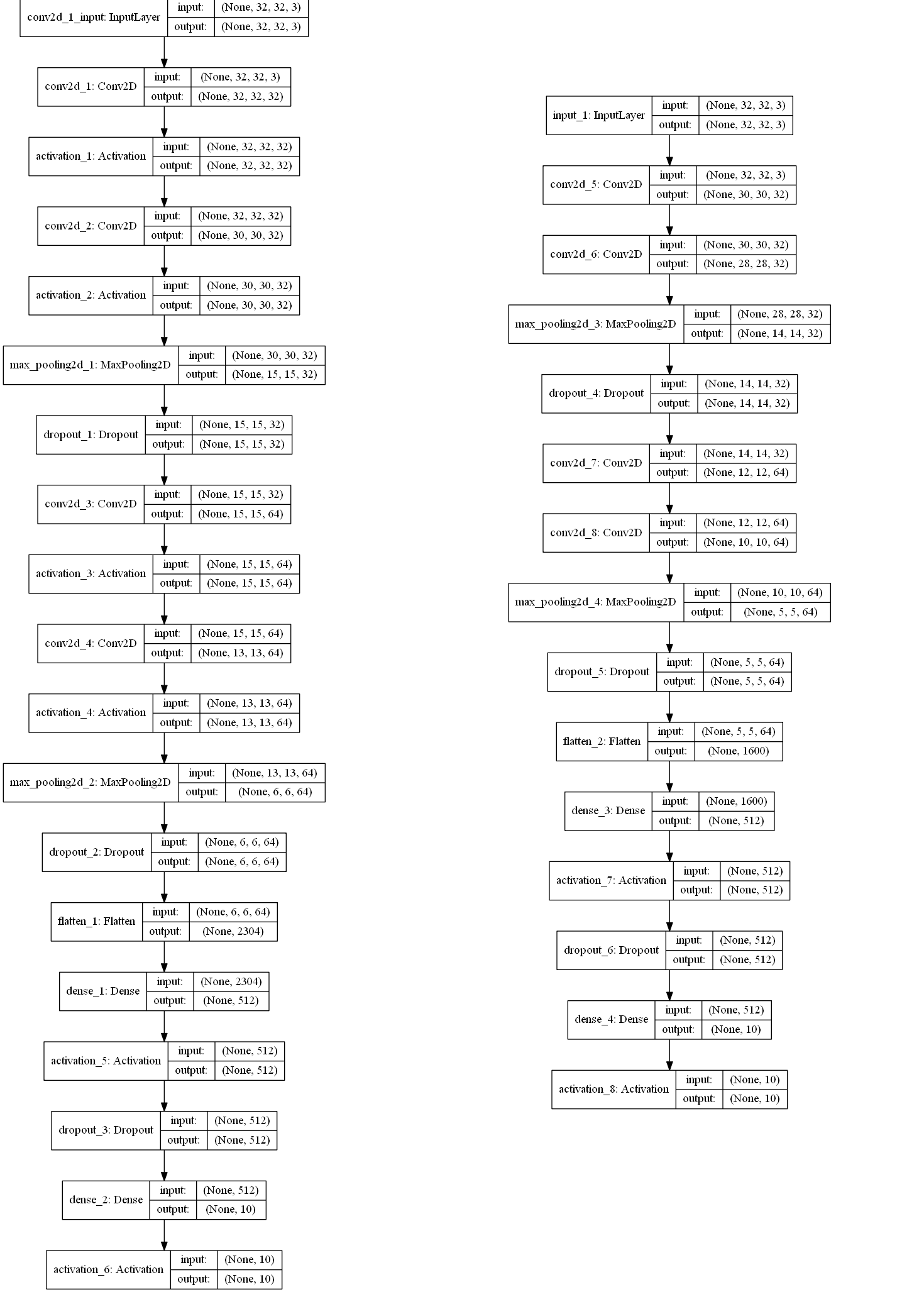
sequence
主要是由于在
x
=
Conv2D(
32
, (
3
,
3
),
activation
=
'relu'
)(inputs)
似乎是将activation合并了,所以model_model更短一些。但是层的结果似乎也是不一样的。这个等到训练结果出来后进一步研究。


目前方向:图像拼接融合、图像识别 联系方式:jsxyhelu@foxmail.com