最近,租房这事儿成了北漂族的一大bug,要想租到称心如意的房子,不仅要眼明手快,还得看清各类“前辈”的评价避开大坑。一位程序员在出行选酒店的时候就借用了程序工具:先用python爬下了海外点评网站TripAdvisor的数千评论,并且用R进行了文本分析和情感分析,科学选房,高效便捷,极具参考价值。
以下,这份超详实的教程拿好不谢。
TripAdvisor提供的信息对于旅行者的出行决策非常重要。但是,要去了解TripAdvisor的泡沫评分和数千个评论文本之间的细微差别是极具挑战性的。
为了更加全面地了解酒店旅客的评论是否会对之后酒店的服务产生影响,我爬取了TripAdvisor中一个名为Hilton Hawaiian Village酒店的所有英文评论。这里我不会对爬虫的细节进行展开。
Python源码:
https://github.com/susanli2016/NLP-with-Python/blob/master/Web%20scraping%20Hilton%20Hawaiian%20Village%20TripAdvisor%20Reviews.py
加载扩展包
library(dplyr)

library(readr)

library(lubridate)

library(ggplot2)

library(tidytext)

library(tidyverse)

library(stringr)

library(tidyr)

library(scales)

library(broom)

library(purrr)

library(widyr)

library(igraph)

library(ggraph)

library(SnowballC)

library(wordcloud)

library(reshape2)

theme_set(theme_minimal())
数据集
df <- read_csv("Hilton_Hawaiian_Village_Waikiki_Beach_Resort-Honolulu_Oahu_Hawaii__en.csv")

df <- df[complete.cases(df), ]

df$review_date <- as.Date(df$review_date, format = "%d-%B-%y")


dim(df); min(df$review_date); max(df$review_date)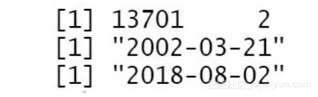
Figure 1
我们在TripAdvisor上一共获得了13,701条关于Hilton Hawaiian Village酒店的英文评论,这些评论的时间范围是从2002–03–21 到2018–08–02。
df %>%

 count(Week = round_date(review_date, "week")) %>%

 ggplot(aes(Week, n)) +

 geom_line() +

 ggtitle('The Number of Reviews Per Week')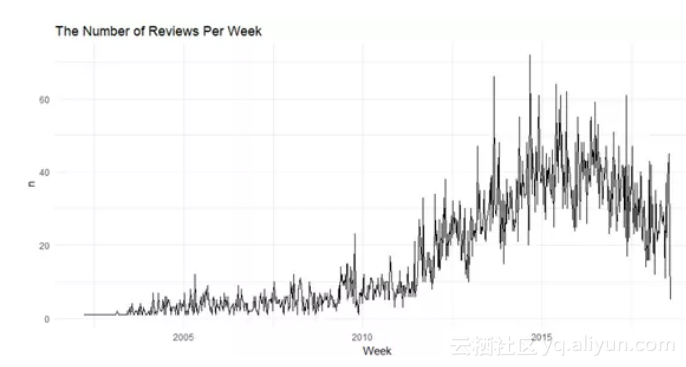
在2014年末,周评论数量达到最高峰。那一个星期里酒店被评论了70次。
对评论文本进行文本挖掘
df <- tibble::rowid_to_column(df, "ID")

df <- df %>%

 mutate(review_date = as.POSIXct(review_date, origin = "1970-01-01"),month = round_date(review_date, "month"))


review_words <- df %>%


 distinct(review_body, .keep_all = TRUE) %>%

 unnest_tokens(word, review_body, drop = FALSE) %>%

 distinct(ID, word, .keep_all = TRUE) %>%

 anti_join(stop_words, by = "word") %>%


 filter(str_detect(word, "[^\\d]")) %>%


 group_by(word) %>%

 mutate(word_total = n()) %>%

 ungroup()


word_counts <- review_words %>%

 count(word, sort = TRUE)


word_counts %>%

 head(25) %>%


 mutate(word = reorder(word, n)) %>%


 ggplot(aes(word, n)) +

 geom_col(fill = "lightblue") +


 scale_y_continuous(labels = comma_format()) +


 coord_flip() +

 labs(title = "Most common words in review text 2002 to date",


 subtitle = "Among 13,701 reviews; stop words removed",


 y = "# of uses")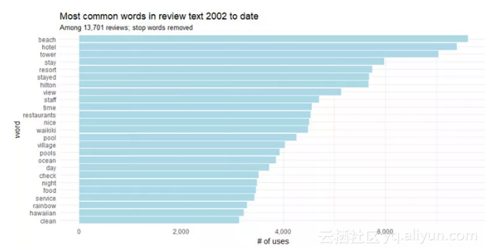
我们还可以更进一步的把“stay”和“stayed”,“pool”和“pools”这些意思相近的词合并起来。这个步骤被称为词干提取,也就是将变形(或是衍生)词语缩减为词干,基词或根词的过程。
word_counts %>%

 head(25) %>%

 mutate(word = wordStem(word)) %>%

 mutate(word = reorder(word, n)) %>%

 ggplot(aes(word, n)) +

 geom_col(fill = "lightblue") +

 scale_y_continuous(labels = comma_format()) +

 coord_flip() +

 labs(title = "Most common words in review text 2002 to date",

 subtitle = "Among 13,701 reviews; stop words removed and stemmed",

 y = "# of uses")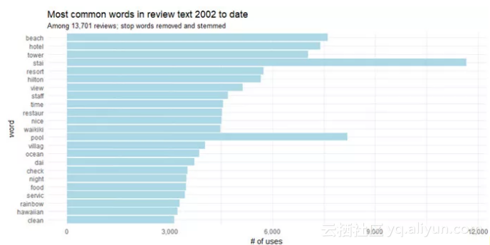
二元词组
通常我们希望了解评论中单词的相互关系。哪些词组在评论文本中比较常用呢?如果给出一列单词,那么后面会随之出现什么单词呢?哪些词之间的关联性最强?许多有意思的文本挖掘都是基于这些关系的。在研究两个连续单词的时候,我们称这些单词对为“二元词组”。
所以,在Hilton Hawaiian Village的评论中,哪些是最常见的二元词组呢?
review_bigrams <- df %>%

 unnest_tokens(bigram, review_body, token = "ngrams", n = 2)


bigrams_separated <- review_bigrams %>%


 separate(bigram, c("word1", "word2"), sep = " ")


bigrams_filtered <- bigrams_separated %>%

 filter(!word1 %in% stop_words$word) %>%

 filter(!word2 %in% stop_words$word)


bigram_counts <- bigrams_filtered %>%

 count(word1, word2, sort = TRUE)


bigrams_united <- bigrams_filtered %>%

 unite(bigram, word1, word2, sep = " ")


bigrams_united %>%

 count(bigram, sort = TRUE)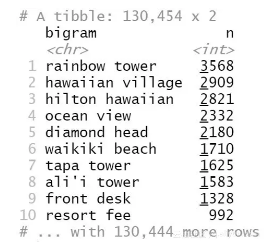
Figure 5
最常见的二元词组是“rainbow tower”(彩虹塔),其次是“hawaiian village”(夏威夷村)。
我们可以利用网络可视化来展示这些二元词组:
review_subject <- df %>%

 unnest_tokens(word, review_body) %>%

 anti_join(stop_words)


my_stopwords <- data_frame(word = c(as.character(1:10)))


review_subject <- review_subject %>%

 anti_join(my_stopwords)


title_word_pairs <- review_subject %>%

 pairwise_count(word, ID, sort = TRUE, upper = FALSE)


set.seed(1234)


title_word_pairs %>%


 filter(n >= 1000) %>%


 graph_from_data_frame() %>%


 ggraph(layout = "fr") +


 geom_edge_link(aes(edge_alpha = n, edge_width = n), edge_colour = "cyan4") +


 geom_node_point(size = 5) +


 geom_node_text(aes(label = name), repel = TRUE,


 point.padding = unit(0.2, "lines")) +


 ggtitle('Word network in TripAdvisor reviews')


 theme_void()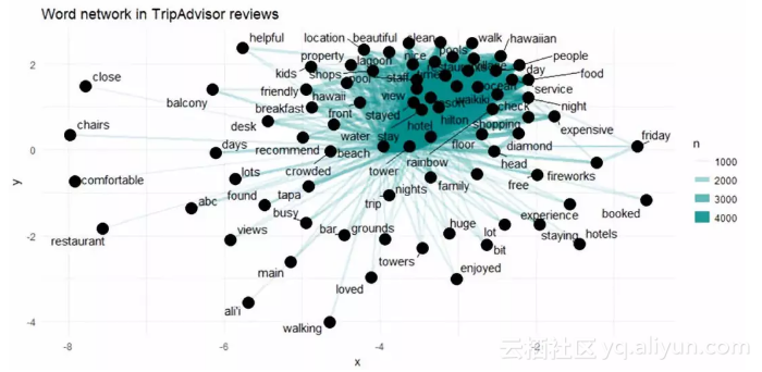
Figure 6
上图展示了TripAdvisor评论中较为常见的二元词组。这些词至少出现了1000次,而且其中不包含停用词。
在网络图中我们发现出现频率最高的几个词存在很强的相关性(“hawaiian”, “village”, “ocean” 和“view”),不过我们没有发现明显的聚集现象。
三元词组
二元词组有时候还不足以说明情况,让我们来看看TripAdvisor中关于Hilton Hawaiian Village酒店最常见的三元词组有哪些。
review_trigrams <- df %>%

 unnest_tokens(trigram, review_body, token = "ngrams", n = 3)


trigrams_separated <- review_trigrams %>%


 separate(trigram, c("word1", "word2", "word3"), sep = " ")


trigrams_filtered <- trigrams_separated %>%

 filter(!word1 %in% stop_words$word) %>%

 filter(!word2 %in% stop_words$word) %>%

 filter(!word3 %in% stop_words$word)


trigram_counts <- trigrams_filtered %>%

 count(word1, word2, word3, sort = TRUE)


trigrams_united <- trigrams_filtered %>%

 unite(trigram, word1, word2, word3, sep = " ")


trigrams_united %>%

 count(trigram, sort = TRUE)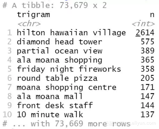
Figure 7
最常见的三元词组是“hilton hawaiian village”,其次是“diamond head tower”,等等。
评论中关键单词的趋势
随着时间的推移,哪些单词或话题变得更加常见,或者更加罕见了呢?从这些信息我们可以探知酒店做出的调整,比如在服务上,翻新上,解决问题上。我们还可以预测哪些主题会更多地被提及。
我们想要解决类似这样的问题:随着时间的推移,在TripAdvisor的评论区中哪些词出现的频率越来越高了?
reviews_per_month <- df %>%

 group_by(month) %>%

 summarize(month_total = n())


word_month_counts <- review_words %>%


 filter(word_total >= 1000) %>%


 count(word, month) %>%


 complete(word, month, fill = list(n = 0)) %>%


 inner_join(reviews_per_month, by = "month") %>%


 mutate(percent = n / month_total) %>%


 mutate(year = year(month) + yday(month) / 365)


mod <- ~ glm(cbind(n, month_total - n) ~ year, ., family = "binomial")


slopes <- word_month_counts %>%

 nest(-word) %>%

 mutate(model = map(data, mod)) %>%


 unnest(map(model, tidy)) %>%


 filter(term == "year") %>%


 arrange(desc(estimate))


slopes %>%

 head(9) %>%


 inner_join(word_month_counts, by = "word") %>%


 mutate(word = reorder(word, -estimate)) %>%


 ggplot(aes(month, n / month_total, color = word)) +

 geom_line(show.legend = FALSE) +

 scale_y_continuous(labels = percent_format()) +

 facet_wrap(~ word, scales = "free_y") +


 expand_limits(y = 0) +


 labs(x = "Year",


 y = "Percentage of reviews containing this word",


 title = "9 fastest growing words in TripAdvisor reviews",


 subtitle = "Judged by growth rate over 15 years")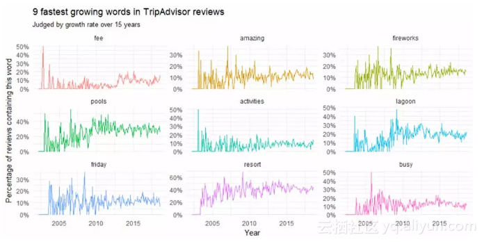
Figure 8
在2010年以前我们可以看到大家讨论的焦点是“friday fireworks”(周五的烟花)和“lagoon”(环礁湖)。而在2005年以前“resort fee”(度假费)和“busy”(繁忙)这些词的词频增长最快。
评论区中哪些词的词频在下降呢?
slopes %>%

 tail(9) %>%

 inner_join(word_month_counts, by = "word") %>%

 mutate(word = reorder(word, estimate)) %>%

 ggplot(aes(month, n / month_total, color = word)) +

 geom_line(show.legend = FALSE) +

 scale_y_continuous(labels = percent_format()) +

 facet_wrap(~ word, scales = "free_y") +

 expand_limits(y = 0) +

 labs(x = "Year",

 y = "Percentage of reviews containing this term",

 title = "9 fastest shrinking words in TripAdvisor reviews",

 subtitle = "Judged by growth rate over 4 years")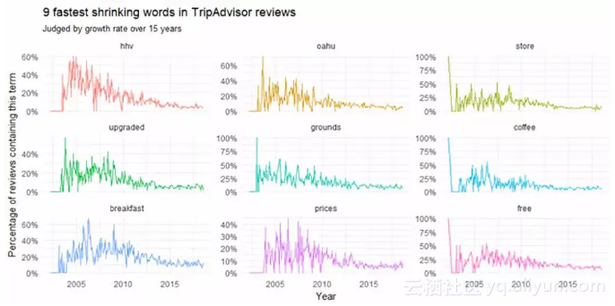
Figure 9
这张图展示了自2010年以来逐渐变少的主题。这些词包括“hhv” (我认为这是 hilton hawaiian village的简称), “breakfast”(早餐), “upgraded”(升级), “prices”(价格) and “free”(免费)。
让我们对一些单词进行比较。
word_month_counts %>%

 filter(word %in% c("service", "food")) %>%

 ggplot(aes(month, n / month_total, color = word)) +

 geom_line(size = 1, alpha = .8) +

 scale_y_continuous(labels = percent_format()) +

 expand_limits(y = 0) +

 labs(x = "Year",

 y = "Percentage of reviews containing this term", title = "service vs food in terms of reviewers interest")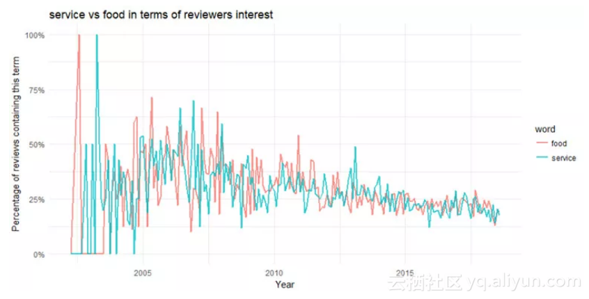
在2010年之前,服务(service)和食物(food)都是热点主题。关于服务和食物的讨论在2003年到达顶峰,自2005年之后就一直在下降,只是偶尔会反弹。
情感分析
情感分析被广泛应用于对评论、调查、网络和社交媒体文本的分析,以反映客户的感受,涉及范围包括市场营销、客户服务和临床医学等。
在本案例中,我们的目标是对评论者(也就是酒店旅客)在住店之后对酒店的态度进行分析。这个态度可能是一个判断或是评价。
下面来看评论中出现得最频繁的积极词汇和消极词汇。
reviews <- df %>%

 filter(!is.na(review_body)) %>%

 select(ID, review_body) %>%

 group_by(row_number()) %>%

 ungroup()

tidy_reviews <- reviews %>%

 unnest_tokens(word, review_body)

tidy_reviews <- tidy_reviews %>%

 anti_join(stop_words)


bing_word_counts <- tidy_reviews %>%


 inner_join(get_sentiments("bing")) %>%


 count(word, sentiment, sort = TRUE) %>%

 ungroup()


bing_word_counts %>%

 group_by(sentiment) %>%

 top_n(10) %>%


 ungroup() %>%


 mutate(word = reorder(word, n)) %>%

 ggplot(aes(word, n, fill = sentiment)) +

 geom_col(show.legend = FALSE) +

 facet_wrap(~sentiment, scales = "free") +


 labs(y = "Contribution to sentiment", x = NULL) +


 coord_flip() +


 ggtitle('Words that contribute to positive and negative sentiment in the reviews')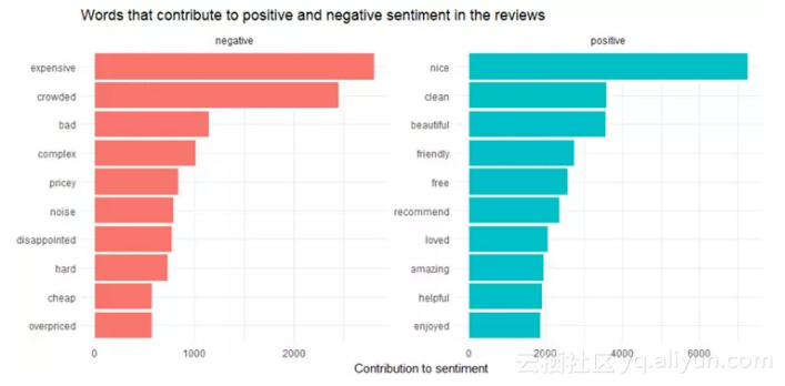
Figure 11
让我们换一个情感文本库,看看结果是否一样。
contributions <- tidy_reviews %>%

 inner_join(get_sentiments("afinn"), by = "word") %>%

 group_by(word) %>%

 summarize(occurences = n(),

 contribution = sum(score))

contributions %>%

 top_n(25, abs(contribution)) %>%

 mutate(word = reorder(word, contribution)) %>%

 ggplot(aes(word, contribution, fill = contribution > 0)) +

 ggtitle('Words with the greatest contributions to positive/negative


 sentiment in reviews') +


 geom_col(show.legend = FALSE) +

 coord_flip()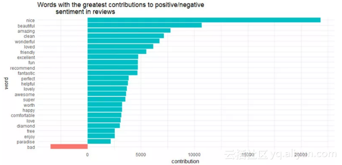
Figure 12
有意思的是,“diamond”(出自“diamond head-钻石头”)被归类为积极情绪。
这里其实有一个潜在问题,比如“clean”(干净)是什么词性取决于语境。如果前面有个“not”(不),这就是一个消极情感了。事实上一元词在否定词(如not)存在的时候经常碰到这种问题,这就引出了我们下一个话题:
在情感分析中使用二元词组来辨明语境
我们想知道哪些词经常前面跟着“not”(不)
bigrams_separated %>%

 filter(word1 == "not") %>%

 count(word1, word2, sort = TRUE)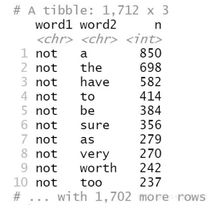
Figure 13
“a”前面跟着“not”的情况出现了850次,而“the”前面跟着“not”出现了698次。不过,这种结果不是特别有实际意义。
AFINN <- get_sentiments("afinn")

not_words <- bigrams_separated %>%

 filter(word1 == "not") %>%

 inner_join(AFINN, by = c(word2 = "word")) %>%

 count(word2, score, sort = TRUE) %>%

 ungroup()


not_words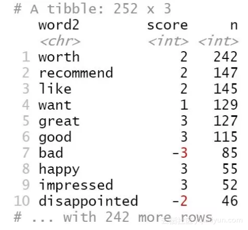
Figure 14
上面的分析告诉我们,在“not”后面最常见的情感词汇是“worth”,其次是“recommend”,这些词都被认为是积极词汇,而且积极程度得分为2。
所以在我们的数据中,哪些单词最容易被误解为相反的情感?
not_words %>%

 mutate(contribution = n * score) %>%

 arrange(desc(abs(contribution))) %>%

 head(20) %>%

 mutate(word2 = reorder(word2, contribution)) %>%

 ggplot(aes(word2, n * score, fill = n * score > 0)) +

 geom_col(show.legend = FALSE) +

 xlab("Words preceded by \"not\"") +

 ylab("Sentiment score * number of occurrences") +

 ggtitle('The 20 words preceded by "not" that had the greatest contribution to


 sentiment scores, positive or negative direction') +


 coord_flip()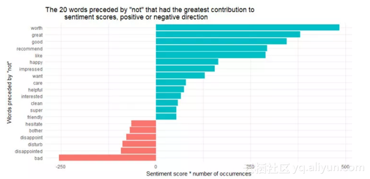
Figure 15
二元词组“not worth”, “not great”, “not good”, “not recommend”和“not like”是导致错误判断的最大根源,使得评论看起来比原来积极的多。
除了“not”以外,还有其他的否定词会对后面的内容进行情绪的扭转,比如“no”, “never” 和“without”。让我们来看一下具体情况。
negation_words <- c("not", "no", "never", "without")


negated_words <- bigrams_separated %>%


 filter(word1 %in% negation_words) %>%

 inner_join(AFINN, by = c(word2 = "word")) %>%


 count(word1, word2, score, sort = TRUE) %>%

 ungroup()


negated_words %>%

 mutate(contribution = n * score,

 word2 = reorder(paste(word2, word1, sep = "__"), contribution)) %>%


 group_by(word1) %>%


 top_n(12, abs(contribution)) %>%


 ggplot(aes(word2, contribution, fill = n * score > 0)) +


 geom_col(show.legend = FALSE) +


 facet_wrap(~ word1, scales = "free") +


 scale_x_discrete(labels = function(x) gsub("__.+$", "", x)) +


 xlab("Words preceded by negation term") +


 ylab("Sentiment score * # of occurrences") +


 ggtitle('The most common positive or negative words to follow negations


 such as "no", "not", "never" and "without"') +


 coord_flip()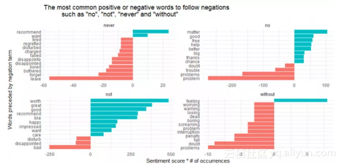
Figure 16
看来导致错判为积极词汇的最大根源来自于“not worth/great/good/recommend”,而另一方面错判为消极词汇的最大根源是“not bad” 和“no problem”。
最后,让我们来观察一下最积极和最消极的评论。
sentiment_messages <- tidy_reviews %>%

 inner_join(get_sentiments("afinn"), by = "word") %>%

 group_by(ID) %>%

 summarize(sentiment = mean(score),

 words = n()) %>%

 ungroup() %>%

 filter(words >= 5)


sentiment_messages %>%


 arrange(desc(sentiment))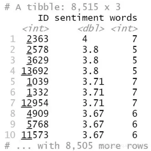
Figure 17
最积极的评论来自于ID为2363的记录:“哇哇哇,这地方太好了!从房间我们可以看到很漂亮的景色,我们住得很开心。Hilton酒店就是很棒!无论是小孩还是大人,这家酒店有着所有你想要的东西。”
df[ which(df$ID==2363), ]$review_body[1]
Figure 18
sentiment_messages %>%

 arrange(sentiment)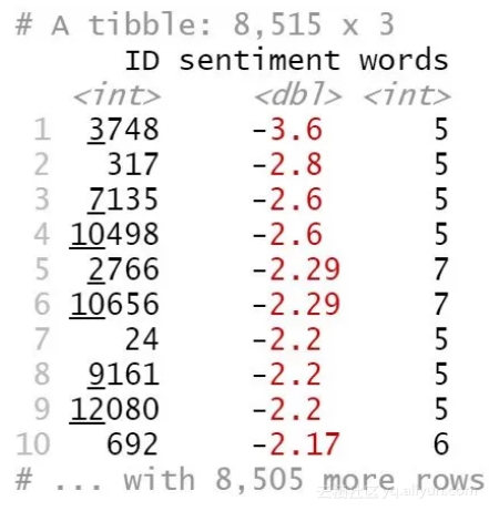
Figure 19
最消极的评论来自于ID为3748的记录:“(我)住了5晚(16年5月12日-5月17日)。第一晚,我们发现地砖坏了,小孩子在玩手指。第二晚,我们看到小蟑螂在儿童食物上爬。前台给我们换了房间,但他们让我们一小时之内搬好房间,否则就不能换房。。。已经晚上11点,我们都很累了,孩子们也睡了。我们拒绝了这个建议。退房的时候,前台小姐跟我讲,蟑螂在他们的旅馆里很常见。她还反问我在加州见不到蟑螂吗?我没想到能在Hilton遇到这样的事情。”
df[ which(df$ID==3748), ]$review_body[1]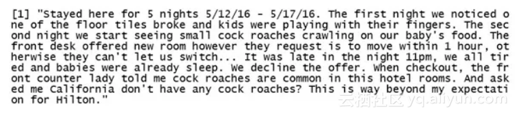
Figure 20
原文发布时间为:2018-09-1
本文作者:Hope、臻臻、CoolBoy