上回书说到(惊堂木!)Dr. Semmelweis and the discovery of handwashing案例中的第8步中使用了bootstrap分析方法(Bootstrap analysis of Semmelweis handwashing data),其实小弟内心写起来是有一丢丢心虚的,因为本身不是相关专业出身没有系统学习过概率学的方法,加之互联网时代大家皮糙肉厚,其实没太多时间仔细研究某一种具体的方式方法(可能只有我一个人这样)。碰巧,今天datacamp里面学习的一章节内容就是根据bootstrap analysis方法展开的。所以趁着工作室打烊前的小空隙,总结一下今天下午的学习成果。
所谓bootstrap analysis:
在统计学中,自助法(Bootstrap Method,Bootstrapping或自助抽样法)是一种从给定训练集中有放回的均匀抽样,也就是说,每当选中一个样本,它等可能地被再次选中并被再次添加到训练集中。自助法由Bradley Efron于1979年在《Annals of Statistics》上发表。当样本来自总体,能以正态分布来描述,其抽样分布(Sampling Distribution)为正态分布(The Normal Distribution);但当样本来自的总体无法以正态分布来描述,则以渐进分析法、自助法等来分析。采用随机可置换抽样(random sampling with replacement)。对于小数据集,自助法效果很好。
via wiki https://zh.wikipedia.org/wiki/%E8%87%AA%E5%8A%A9%E6%B3%95
测试一下你对上文阅读理解能力:
Q:What is a bootstrap replicate?
A:A single value of a statistic computed from a bootstrap sample.
Q:How many unique bootstrap samples can be drawn (e.g.,
[-1, 0, 1]and[1, 0, -1]areunique), and what is the maximum mean you can get from a bootstrap sample?A:There are 27 unique samples, and the maximum mean is 1.
为了更方便大家理解datacamp的老师们以谢菲尔德气象站从1883年到2015年的气象数据(伦敦的降雨情况)(导入numpy的rainfall中)为例作以分析:
for i in range(50):#做50次实验
    # Generate bootstrap sample: bs_sample
    bs_sample = np.random.choice(rainfall, size=len(rainfall))#每次有放回地抽取一个和rainfall一样长的样本bs_sample

    # Compute and plot ECDF from bootstrap sample
    x, y = ecdf(bs_sample)#为bs_sample生成一个CDF(累计密度函数),返回x值是降雨量,y值是小于这个x值的概率
    _ = plt.plot(x, y, marker='.', linestyle='none',
                 c='gray', alpha=0.1)#将这次循环中的bs_sample(i)画在图上

# Compute and plot ECDF from original data
x, y = ecdf(rainfall)#为真实值生成一个CDF
_ = plt.plot(x, y, marker='.')#也画在图上

# Make margins and label axes
plt.margins(0.02)
_ = plt.xlabel('yearly rainfall (mm)')
_ = plt.ylabel('ECDF')

# Show the plot
plt.show()
output:
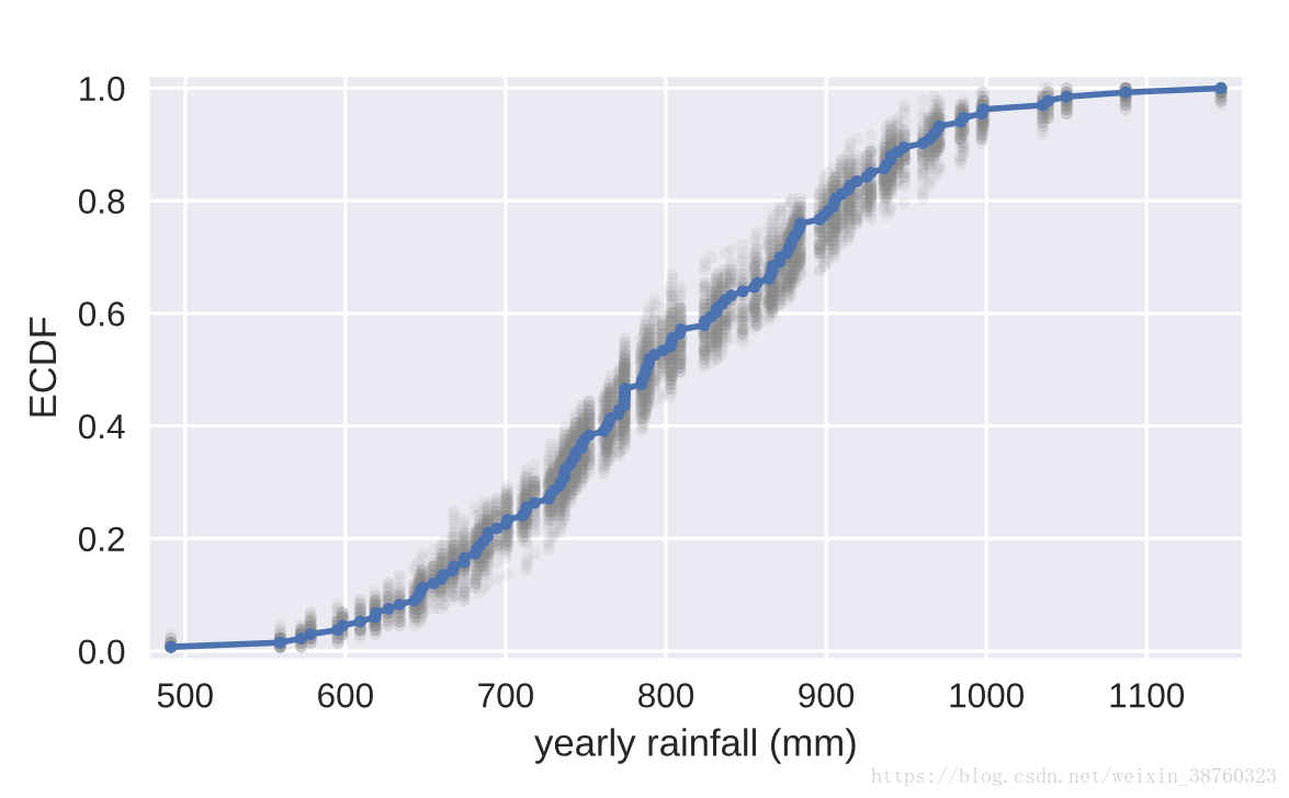
看见那些模模糊糊的小黑影了吗,这些是你经过bootstrap replicate出来的结果,可以看出replicate出来的数据在一定程度上符合真实数据的概率分布,这就为我们下一步开展工作奠定了基础。
By graphically displaying the bootstrap samples with an ECDF, you can get a feel for how bootstrap sampling allows probabilistic descriptions of data.
可是这些sample真的可信吗?我们继续分析:
为了后面应用方便,我们定义下面函数:
def bootstrap_replicate_1d(data,func):
	bs_sample=np.random.choice(data,len(data))
	return func(bs_sample)
#产生一次bootstrap sample,并对这个sample进行一次func操作
def draw_bs_reps(data,func,size=1):
bs_replicates=np.empty(size)
for i in range(size):
bs_replicates[i]=bootstrap_replicate_1d(data,func)
return bs_replicates
#重复size次bootstrap_replicate_1d从函数bootstrap_replicate_1d的功能上看,它sample了一个样本,而后返回了对这个样本的某种处理(func)
draw_bs_reps函数则是对bootstrap sample进行重复,并将返回值记录在案,绳之以法,并最终返回案底。
那么这两个函数(实际上是draw_bs_reps)怎么用呢?
# Take 10,000 bootstrap replicates of the mean: bs_replicates
bs_replicates = draw_bs_reps(rainfall,np.mean,size=10000)#将rainfall做bootstrap sample,并将结果均值,重复10000次

# Compute and print SEM
sem = np.std(rainfall) / np.sqrt(len(rainfall))#求出rainfall真实值的标准差
print(sem)
# Compute and print standard deviation of bootstrap replicates
bs_std = np.std(bs_replicates)#输出10000次平均值的标准差
print(bs_std)

# Make a histogram of the results
_ = plt.hist(bs_replicates, bins=50, normed=True)#做10000次实验的概率直方图
_ = plt.xlabel('mean annual rainfall (mm)')
_ = plt.ylabel('PDF')

# Show the plot
plt.show()
output:
10.5105491505
10.4659270712
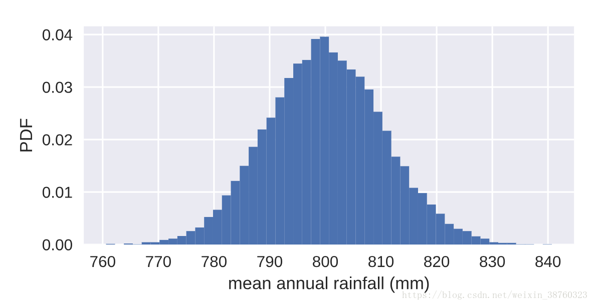
可以看出真实值的离散程度和做10000次实验得出的平均值的离散程度是非常接近的。
而且当做100000次实验的时候,两者的离散程度就愈发接近了。
10.5105491505
10.5062818229
这能说明什么呢?
当我们做一个统计计算时,经常会发现无法收集到全部的样本数据(从盘古开天辟地到宇宙大撕裂的降雨情况),出于这种无奈,我们只好退而求其次地相信选取其中的某一段数据(1883年到2015年),经过反复的bootstrap replicate(相当于无限重复抽样的次数,以弥补我们在客观现实世界中无法发无限次重复实验的遗憾),得到一系列的样本,从中认为这就是最接近客观世界的样本。
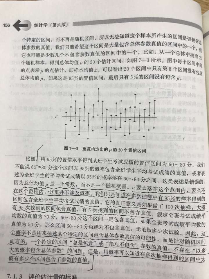
If we repeated measurements over and over again,p% of the observed values would lie within the p%confidence interval.
如果我们依次便吹牛逼说自己得到了某一个准确的值,它便是客观世界中(从盘古开天辟地到宇宙大撕裂的时期的)降雨的平均值(或者方差,或者其他统计数据),那确实显得有点扯了。于使统计学家们经过不懈努力定义了一个置信区间,认为如果在这种抽样操作不变的情况下,再进行的所有抽样,其平均值(或者其他统计数据)落在这个区间内的是有一定可能性的(95%,或者其他)。
np.percentile(bs_replicates,[2.5,97.5])emergency!!!(存疑)
今天刚查了一下percentile的用法,发现它只是取数据在升序排列后位于2.5%位置和97.5%位置的,并不是我们传统意义上的对正态分布(或小样本T分布所求的置信区间)。
应用scipy求一个小样本的T分布置信区间代码如下:
import numpy as np
from scipy import stats

X1=np.array([14.65,14.95,8.49,9.51,10.23,2.75])
Xmean=X1.mean()
Xstd=X1.std(ddof=1)
interval=stats.t.interval(0.95,len(X1-1),Xmean,Xstd)

print("置信区间为:",interval)
https://blog.csdn.net/brucewong0516/article/details/80205422
回复上面的疑问!!!!!!
刚刚跟大神聊了一下,得到的回复如下:
基于t分布的均值置信区间估计是在正态总体假设下才能用的,而百分位法没这个限制,这也和Bootstrap法不假设样本的分布类型相匹配
并且还得知:
是的,Bootstrsp方法只能缩减置信区间,无法更加准确的估计客观真实值,这是小样本的根本缺陷,如果想更加准确的估计客观真实值,就只能增大样本容量。
而且Bootstrap方法得到的置信区间是用百分位法得到的,和正态总体假设的t分布法不一样
恍然大悟啊有木有!
output:
array([ 779.76992481, 820.95043233])
置信区间参考:https://www.zhihu.com/question/26419030
我认为这个解释是最为靠谱的:
然后我们用同样的方法对方差进行了估计:
# Generate 10,000 bootstrap replicates of the variance: bs_replicates
bs_replicates = draw_bs_reps(rainfall,np.var,10000)#对10000次实验求方差

# Put the variance in units of square centimeters
bs_replicates=bs_replicates/100

# Make a histogram of the results
_ = plt.hist(bs_replicates, bins=50, normed=True)
_ = plt.xlabel('variance of annual rainfall (sq. cm)')
_ = plt.ylabel('PDF')

# Show the plot
plt.show()
output:
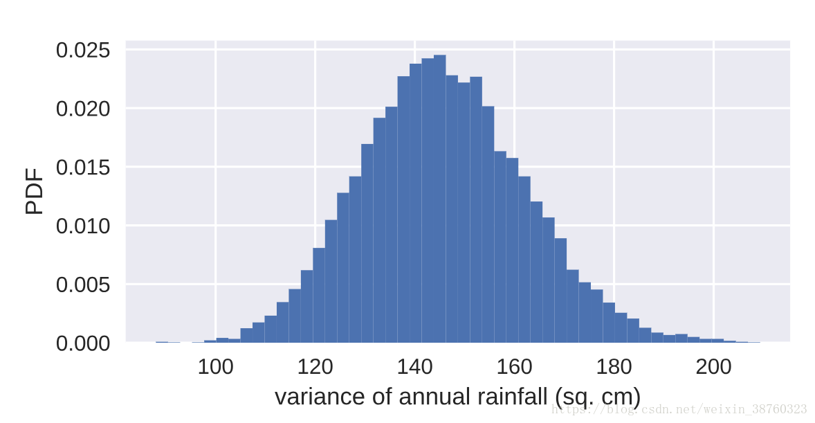
当然也可以对其他案例进行分析,案例暂且不表,只贴出一下结果:
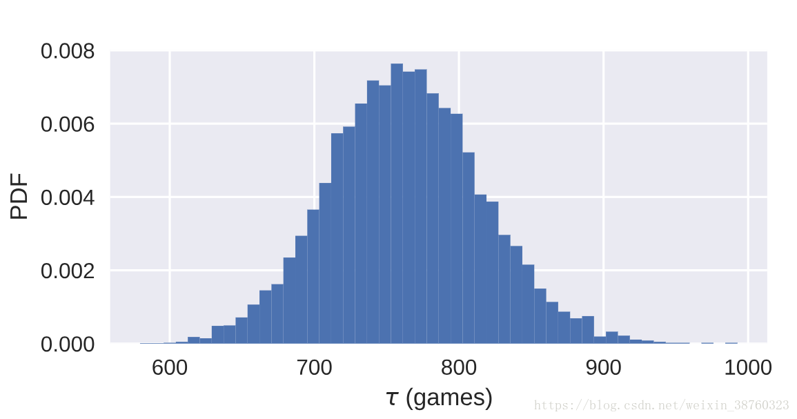
# Draw bootstrap replicates of the mean no-hitter time (equal to tau): bs_replicates
bs_replicates = draw_bs_reps(nohitter_times,np.mean,10000)

# Compute the 95% confidence interval: conf_int
conf_int = np.percentile(bs_replicates,[2.5,97.5])

# Print the confidence interval
print('95% confidence interval =', conf_int, 'games')

# Plot the histogram of the replicates
_ = plt.hist(bs_replicates, bins=50, normed=True)
_ = plt.xlabel(r'$\tau$ (games)')
_ = plt.ylabel('PDF')

# Show the plot
plt.show()
output:
95% confidence interval = [ 660.67280876 871.63077689] games
以上的分析为均为一种nonparametric inference(非参数估计,Make no assumptions about the model orprobability distribution underlying the data,参考:https://blog.csdn.net/drrlalala/article/details/45533821 ,已知样本所属的类别,但未知总体概率密度函数的形式,要求我们直接推断概率密度函数本身。非参数估计也有人将其称之为无参密度估计,它是一种对先验知识要求最少,完全依靠训练数据进行估计,而且可以用于任意形状密度估计的方法。)下面介绍一些参数估计的方法,还是二维参数(paris bootstrap)。
这个例子是关于奥巴马2008年大选(2008 US swing state election results),我们要完成的是将各个洲的选票数与奥巴马的得票比作以拟合(从而实现预测?maybe)。
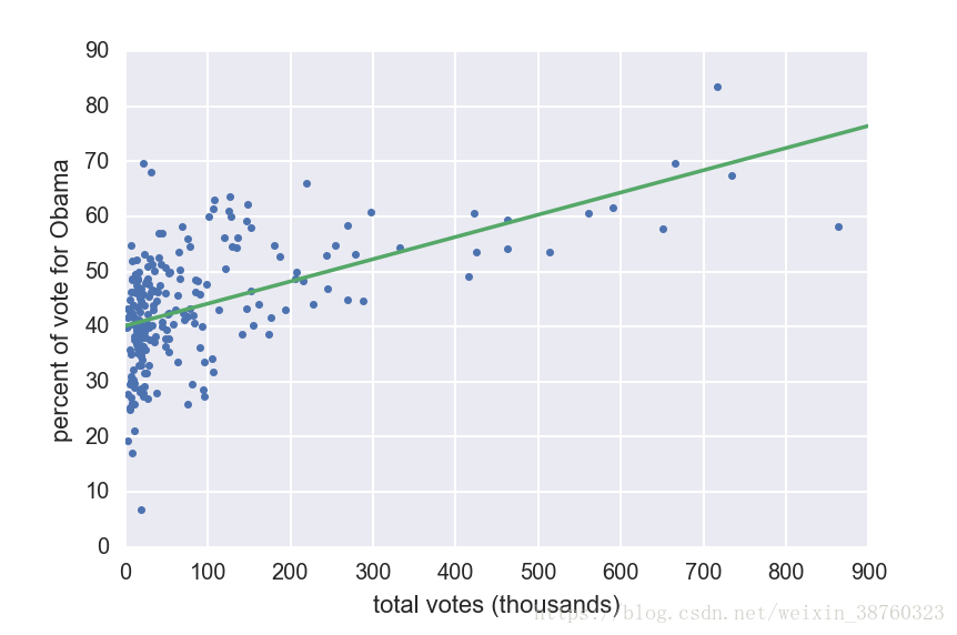
与之前不同之处是,变量从前一个例子中的单一变量(降雨量)变成了两个变量(选票数与得票比),而np.random.choice只能针对单一变量进行抽样,而数据是成对(in pair)出现的,这意味着我们不能像之前一样sample得简单粗暴。看一看这个案例中我们是如何进行抽样的:
def draw_bs_pairs_linreg(x, y, size=1):
    """Perform pairs bootstrap for linear regression."""

    # Set up array of indices to sample from: inds
    inds = np.arange(len(x))#选用pair中的一个变量长度作为指数

    # Initialize replicates: bs_slope_reps, bs_intercept_reps
    bs_slope_reps = np.empty(size)#初始化两个空list用于存储每次实验得到的参数
    bs_intercept_reps = np.empty(size)

    # Generate replicates
    for i in range(size):#重复size次实验
        bs_inds = np.random.choice(inds, size=len(inds))#抽取和变量长度相当个数的指数
        bs_x, bs_y = x[bs_inds], y[bs_inds]#依据指数选取成对的变量
        bs_slope_reps[i], bs_intercept_reps[i] = np.polyfit(bs_x,bs_y,1)#用选取到的变量进行线性拟合

    return bs_slope_reps, bs_intercept_reps#返回斜率和截距
案例中利用新定义的指数作为抽取哪些变量的计量,完成了bootstrap sample的过程。
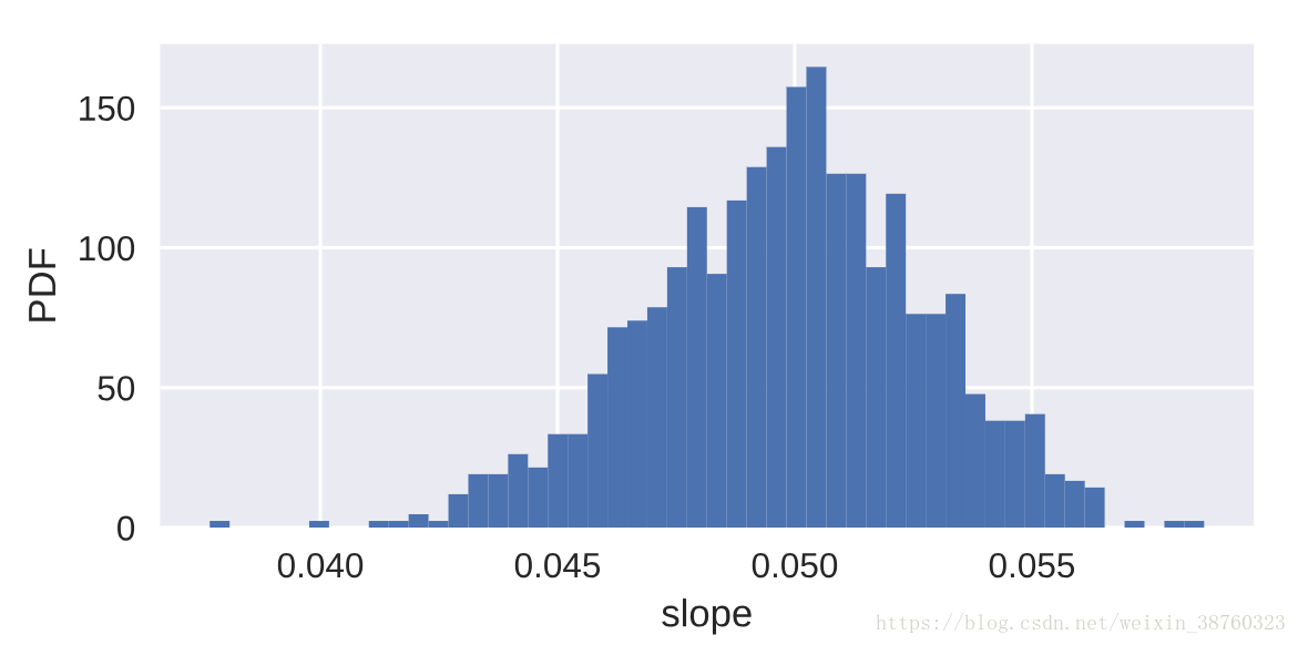
然鹅,datacamp的老师并没有继续使用奥巴马的案例完成后面的工作,而是选用了之前妇女生育率和文盲率的案例进行分析(- - 我也没看懂),不过代码大致是相同的:
# Generate replicates of slope and intercept using pairs bootstrap
bs_slope_reps, bs_intercept_reps = draw_bs_pairs_linreg(illiteracy,fertility,1000)

# Compute and print 95% CI for slope
print(np.percentile(bs_slope_reps, [2.5,97.5]))

# Plot the histogram
_ = plt.hist(bs_slope_reps, bins=50, normed=True)
_ = plt.xlabel('slope')
_ = plt.ylabel('PDF')
plt.show()
output:
[ 0.04378061 0.0551616 ]
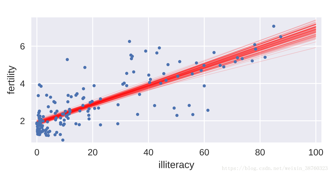
# Generate array of x-values for bootstrap lines: x
x = np.array([0,100])

# Plot the bootstrap lines
for i in range(100):
    _ = plt.plot(x, bs_slope_reps[i]*x + bs_intercept_reps[i],
                 linewidth=0.5, alpha=0.2, color='red')

# Plot the data
_ = plt.plot(illiteracy,fertility,marker='.',linestyle='none')

# Label axes, set the margins, and show the plot
_ = plt.xlabel('illiteracy')
_ = plt.ylabel('fertility')
plt.margins(0.02)
plt.show()
output:
thats all thank you~
课程讲义:https://github.com/chenchutong/DESOLATION_ROW/blob/master/slides/ch2_slides.pdf
