鸢尾花分类预测数据分析
- 目标:根据未知种类鸢尾花的特征预测其种类
- 数据:鸢尾花数据集
- 分析:
- 描述性分析
- 探索性分析
- 建模分析
- 模型分析
- 迭代分析
- 成果:位置种类鸢尾花的预测结果
import numpy as np
import matplotlib.pyplot as plt
# import pandas as pd
from sklearn import neighbors, datasets
加载鸢尾花数据集
iris = datasets.load_iris()
iris
{'DESCR': 'Iris Plants Database\n====================\n\nNotes\n-----\nData Set Characteristics:\n :Number of Instances: 150 (50 in each of three classes)\n :Number of Attributes: 4 numeric, predictive attributes and the class\n :Attribute Information:\n - sepal length in cm\n - sepal width in cm\n - petal length in cm\n - petal width in cm\n - class:\n - Iris-Setosa\n - Iris-Versicolour\n - Iris-Virginica\n :Summary Statistics:\n\n ============== ==== ==== ======= ===== ====================\n Min Max Mean SD Class Correlation\n ============== ==== ==== ======= ===== ====================\n sepal length: 4.3 7.9 5.84 0.83 0.7826\n sepal width: 2.0 4.4 3.05 0.43 -0.4194\n petal length: 1.0 6.9 3.76 1.76 0.9490 (high!)\n petal width: 0.1 2.5 1.20 0.76 0.9565 (high!)\n ============== ==== ==== ======= ===== ====================\n\n :Missing Attribute Values: None\n :Class Distribution: 33.3% for each of 3 classes.\n :Creator: R.A. Fisher\n :Donor: Michael Marshall (MARSHALL%PLU@io.arc.nasa.gov)\n :Date: July, 1988\n\nThis is a copy of UCI ML iris datasets.\nhttp://archive.ics.uci.edu/ml/datasets/Iris\n\nThe famous Iris database, first used by Sir R.A Fisher\n\nThis is perhaps the best known database to be found in the\npattern recognition literature. Fisher\'s paper is a classic in the field and\nis referenced frequently to this day. (See Duda & Hart, for example.) The\ndata set contains 3 classes of 50 instances each, where each class refers to a\ntype of iris plant. One class is linearly separable from the other 2; the\nlatter are NOT linearly separable from each other.\n\nReferences\n----------\n - Fisher,R.A. "The use of multiple measurements in taxonomic problems"\n Annual Eugenics, 7, Part II, 179-188 (1936); also in "Contributions to\n Mathematical Statistics" (John Wiley, NY, 1950).\n - Duda,R.O., & Hart,P.E. (1973) Pattern Classification and Scene Analysis.\n (Q327.D83) John Wiley & Sons. ISBN 0-471-22361-1. See page 218.\n - Dasarathy, B.V. (1980) "Nosing Around the Neighborhood: A New System\n Structure and Classification Rule for Recognition in Partially Exposed\n Environments". IEEE Transactions on Pattern Analysis and Machine\n Intelligence, Vol. PAMI-2, No. 1, 67-71.\n - Gates, G.W. (1972) "The Reduced Nearest Neighbor Rule". IEEE Transactions\n on Information Theory, May 1972, 431-433.\n - See also: 1988 MLC Proceedings, 54-64. Cheeseman et al"s AUTOCLASS II\n conceptual clustering system finds 3 classes in the data.\n - Many, many more ...\n',
'data': array([[ 5.1, 3.5, 1.4, 0.2],
[ 4.9, 3. , 1.4, 0.2],
[ 4.7, 3.2, 1.3, 0.2],
[ 4.6, 3.1, 1.5, 0.2],
[ 5. , 3.6, 1.4, 0.2],
[ 5.4, 3.9, 1.7, 0.4],
[ 4.6, 3.4, 1.4, 0.3],
[ 5. , 3.4, 1.5, 0.2],
[ 4.4, 2.9, 1.4, 0.2],
[ 4.9, 3.1, 1.5, 0.1],
[ 5.4, 3.7, 1.5, 0.2],
[ 4.8, 3.4, 1.6, 0.2],
[ 4.8, 3. , 1.4, 0.1],
[ 4.3, 3. , 1.1, 0.1],
[ 5.8, 4. , 1.2, 0.2],
[ 5.7, 4.4, 1.5, 0.4],
[ 5.4, 3.9, 1.3, 0.4],
[ 5.1, 3.5, 1.4, 0.3],
[ 5.7, 3.8, 1.7, 0.3],
[ 5.1, 3.8, 1.5, 0.3],
[ 5.4, 3.4, 1.7, 0.2],
[ 5.1, 3.7, 1.5, 0.4],
[ 4.6, 3.6, 1. , 0.2],
[ 5.1, 3.3, 1.7, 0.5],
[ 4.8, 3.4, 1.9, 0.2],
[ 5. , 3. , 1.6, 0.2],
[ 5. , 3.4, 1.6, 0.4],
[ 5.2, 3.5, 1.5, 0.2],
[ 5.2, 3.4, 1.4, 0.2],
[ 4.7, 3.2, 1.6, 0.2],
[ 4.8, 3.1, 1.6, 0.2],
[ 5.4, 3.4, 1.5, 0.4],
[ 5.2, 4.1, 1.5, 0.1],
[ 5.5, 4.2, 1.4, 0.2],
[ 4.9, 3.1, 1.5, 0.1],
[ 5. , 3.2, 1.2, 0.2],
[ 5.5, 3.5, 1.3, 0.2],
[ 4.9, 3.1, 1.5, 0.1],
[ 4.4, 3. , 1.3, 0.2],
[ 5.1, 3.4, 1.5, 0.2],
[ 5. , 3.5, 1.3, 0.3],
[ 4.5, 2.3, 1.3, 0.3],
[ 4.4, 3.2, 1.3, 0.2],
[ 5. , 3.5, 1.6, 0.6],
[ 5.1, 3.8, 1.9, 0.4],
[ 4.8, 3. , 1.4, 0.3],
[ 5.1, 3.8, 1.6, 0.2],
[ 4.6, 3.2, 1.4, 0.2],
[ 5.3, 3.7, 1.5, 0.2],
[ 5. , 3.3, 1.4, 0.2],
[ 7. , 3.2, 4.7, 1.4],
[ 6.4, 3.2, 4.5, 1.5],
[ 6.9, 3.1, 4.9, 1.5],
[ 5.5, 2.3, 4. , 1.3],
[ 6.5, 2.8, 4.6, 1.5],
[ 5.7, 2.8, 4.5, 1.3],
[ 6.3, 3.3, 4.7, 1.6],
[ 4.9, 2.4, 3.3, 1. ],
[ 6.6, 2.9, 4.6, 1.3],
[ 5.2, 2.7, 3.9, 1.4],
[ 5. , 2. , 3.5, 1. ],
[ 5.9, 3. , 4.2, 1.5],
[ 6. , 2.2, 4. , 1. ],
[ 6.1, 2.9, 4.7, 1.4],
[ 5.6, 2.9, 3.6, 1.3],
[ 6.7, 3.1, 4.4, 1.4],
[ 5.6, 3. , 4.5, 1.5],
[ 5.8, 2.7, 4.1, 1. ],
[ 6.2, 2.2, 4.5, 1.5],
[ 5.6, 2.5, 3.9, 1.1],
[ 5.9, 3.2, 4.8, 1.8],
[ 6.1, 2.8, 4. , 1.3],
[ 6.3, 2.5, 4.9, 1.5],
[ 6.1, 2.8, 4.7, 1.2],
[ 6.4, 2.9, 4.3, 1.3],
[ 6.6, 3. , 4.4, 1.4],
[ 6.8, 2.8, 4.8, 1.4],
[ 6.7, 3. , 5. , 1.7],
[ 6. , 2.9, 4.5, 1.5],
[ 5.7, 2.6, 3.5, 1. ],
[ 5.5, 2.4, 3.8, 1.1],
[ 5.5, 2.4, 3.7, 1. ],
[ 5.8, 2.7, 3.9, 1.2],
[ 6. , 2.7, 5.1, 1.6],
[ 5.4, 3. , 4.5, 1.5],
[ 6. , 3.4, 4.5, 1.6],
[ 6.7, 3.1, 4.7, 1.5],
[ 6.3, 2.3, 4.4, 1.3],
[ 5.6, 3. , 4.1, 1.3],
[ 5.5, 2.5, 4. , 1.3],
[ 5.5, 2.6, 4.4, 1.2],
[ 6.1, 3. , 4.6, 1.4],
[ 5.8, 2.6, 4. , 1.2],
[ 5. , 2.3, 3.3, 1. ],
[ 5.6, 2.7, 4.2, 1.3],
[ 5.7, 3. , 4.2, 1.2],
[ 5.7, 2.9, 4.2, 1.3],
[ 6.2, 2.9, 4.3, 1.3],
[ 5.1, 2.5, 3. , 1.1],
[ 5.7, 2.8, 4.1, 1.3],
[ 6.3, 3.3, 6. , 2.5],
[ 5.8, 2.7, 5.1, 1.9],
[ 7.1, 3. , 5.9, 2.1],
[ 6.3, 2.9, 5.6, 1.8],
[ 6.5, 3. , 5.8, 2.2],
[ 7.6, 3. , 6.6, 2.1],
[ 4.9, 2.5, 4.5, 1.7],
[ 7.3, 2.9, 6.3, 1.8],
[ 6.7, 2.5, 5.8, 1.8],
[ 7.2, 3.6, 6.1, 2.5],
[ 6.5, 3.2, 5.1, 2. ],
[ 6.4, 2.7, 5.3, 1.9],
[ 6.8, 3. , 5.5, 2.1],
[ 5.7, 2.5, 5. , 2. ],
[ 5.8, 2.8, 5.1, 2.4],
[ 6.4, 3.2, 5.3, 2.3],
[ 6.5, 3. , 5.5, 1.8],
[ 7.7, 3.8, 6.7, 2.2],
[ 7.7, 2.6, 6.9, 2.3],
[ 6. , 2.2, 5. , 1.5],
[ 6.9, 3.2, 5.7, 2.3],
[ 5.6, 2.8, 4.9, 2. ],
[ 7.7, 2.8, 6.7, 2. ],
[ 6.3, 2.7, 4.9, 1.8],
[ 6.7, 3.3, 5.7, 2.1],
[ 7.2, 3.2, 6. , 1.8],
[ 6.2, 2.8, 4.8, 1.8],
[ 6.1, 3. , 4.9, 1.8],
[ 6.4, 2.8, 5.6, 2.1],
[ 7.2, 3. , 5.8, 1.6],
[ 7.4, 2.8, 6.1, 1.9],
[ 7.9, 3.8, 6.4, 2. ],
[ 6.4, 2.8, 5.6, 2.2],
[ 6.3, 2.8, 5.1, 1.5],
[ 6.1, 2.6, 5.6, 1.4],
[ 7.7, 3. , 6.1, 2.3],
[ 6.3, 3.4, 5.6, 2.4],
[ 6.4, 3.1, 5.5, 1.8],
[ 6. , 3. , 4.8, 1.8],
[ 6.9, 3.1, 5.4, 2.1],
[ 6.7, 3.1, 5.6, 2.4],
[ 6.9, 3.1, 5.1, 2.3],
[ 5.8, 2.7, 5.1, 1.9],
[ 6.8, 3.2, 5.9, 2.3],
[ 6.7, 3.3, 5.7, 2.5],
[ 6.7, 3. , 5.2, 2.3],
[ 6.3, 2.5, 5. , 1.9],
[ 6.5, 3. , 5.2, 2. ],
[ 6.2, 3.4, 5.4, 2.3],
[ 5.9, 3. , 5.1, 1.8]]),
'feature_names': ['sepal length (cm)',
'sepal width (cm)',
'petal length (cm)',
'petal width (cm)'],
'target': array([0, 0, 0, 0, 0, 0, 0, 0, 0, 0, 0, 0, 0, 0, 0, 0, 0, 0, 0, 0, 0, 0, 0,
0, 0, 0, 0, 0, 0, 0, 0, 0, 0, 0, 0, 0, 0, 0, 0, 0, 0, 0, 0, 0, 0, 0,
0, 0, 0, 0, 1, 1, 1, 1, 1, 1, 1, 1, 1, 1, 1, 1, 1, 1, 1, 1, 1, 1, 1,
1, 1, 1, 1, 1, 1, 1, 1, 1, 1, 1, 1, 1, 1, 1, 1, 1, 1, 1, 1, 1, 1, 1,
1, 1, 1, 1, 1, 1, 1, 1, 2, 2, 2, 2, 2, 2, 2, 2, 2, 2, 2, 2, 2, 2, 2,
2, 2, 2, 2, 2, 2, 2, 2, 2, 2, 2, 2, 2, 2, 2, 2, 2, 2, 2, 2, 2, 2, 2,
2, 2, 2, 2, 2, 2, 2, 2, 2, 2, 2, 2]),
'target_names': array(['setosa', 'versicolor', 'virginica'],
dtype='<U10')}
数据认知
type(iris)sklearn.datasets.base.Bunch
数据集,样本150个
150行,4列
'data':array([
  [ 5.1,  3.5,  1.4,  0.2],
  [ 4.9,  3. ,  1.4,  0.2],
  [ 4.7,  3.2,  1.3,  0.2],
  [ 4.6,  3.1,  1.5,  0.2],
  [ 5. ,  3.6,  1.4,  0.2],
  [ 5.4,  3.9,  1.7,  0.4],
  ...
])
特征:4个
'feature_names': [
  'sepal length (cm)', #花萼长度
  'sepal width (cm)', #花萼宽度
  'petal length (cm)', #花瓣长度
  'petal width (cm)' #花瓣宽度
],
结果
标签1个:1行,150列
'target': array([
  0, 0, 0... 1, 1, 1... 2, 2, 2...
])
结果对应
'target_names': array([
  'setosa', # 0 山鸢尾
  'versicolor', # 1 变色鸢尾
  'virginica' # 2 维吉尼亚鸢尾
]}
描述性分析
se = iris.data[0:50] # 山鸢尾特征,50行
ve = iris.data[50:100] # 变色鸢尾特征,50行
vi = iris.data[100:150] # 维吉尼亚特征,50行
se

comb = [[0,1],[0,2],[0,3],[1,2],[1,3],[2,3]] #二维图像,4个特征两两组合

se[:,comb[0][0]] # 山鸢尾特征1,花萼长
array([ 5.1, 4.9, 4.7, 4.6, 5. , 5.4, 4.6, 5. , 4.4, 4.9, 5.4,
4.8, 4.8, 4.3, 5.8, 5.7, 5.4, 5.1, 5.7, 5.1, 5.4, 5.1,
4.6, 5.1, 4.8, 5. , 5. , 5.2, 5.2, 4.7, 4.8, 5.4, 5.2,
5.5, 4.9, 5. , 5.5, 4.9, 4.4, 5.1, 5. , 4.5, 4.4, 5. ,
5.1, 4.8, 5.1, 4.6, 5.3, 5. ])
图像绘制
plt.figure(1, figsize=(18,10))

for i in range(6):
    plt.subplot(231+i)
    plt.plot(se[:,comb[i][0]],se[:,comb[i][1]],'o',color='#ff0000')
    plt.plot(ve[:,comb[i][0]],ve[:,comb[i][1]],'^',color='#00ff00')
    plt.plot(vi[:,comb[i][0]],vi[:,comb[i][1]],'+',color='#ff00ff')

plt.show()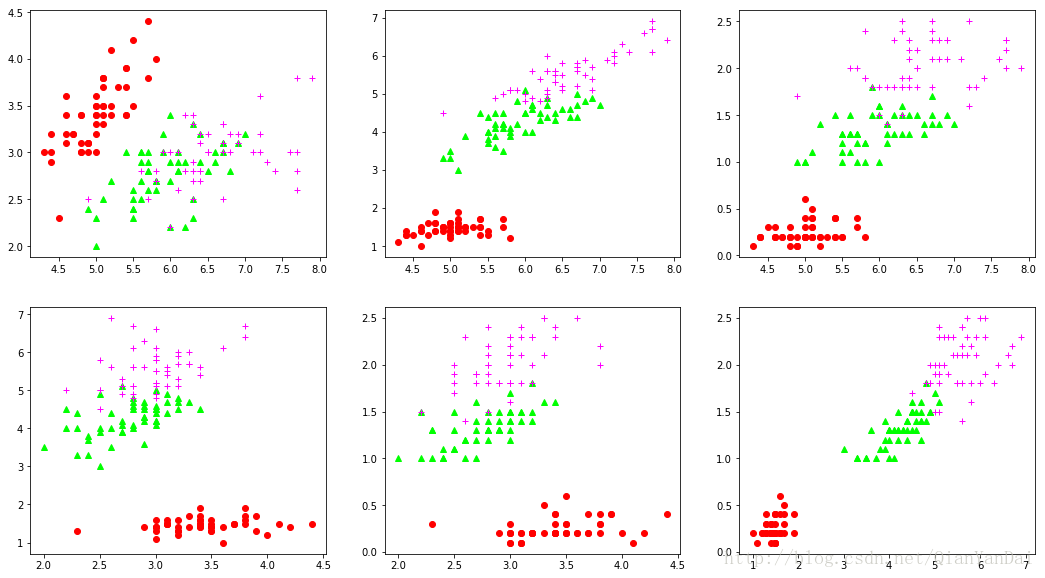
探索性分析
建模分析
# x轴,训练数据
x = iris.data
x
array([[ 5.1, 3.5, 1.4, 0.2],
[ 4.9, 3. , 1.4, 0.2],
[ 4.7, 3.2, 1.3, 0.2],
[ 4.6, 3.1, 1.5, 0.2],
[ 5. , 3.6, 1.4, 0.2],
[ 5.4, 3.9, 1.7, 0.4],
[ 4.6, 3.4, 1.4, 0.3],
[ 5. , 3.4, 1.5, 0.2],
[ 4.4, 2.9, 1.4, 0.2],
[ 4.9, 3.1, 1.5, 0.1],
[ 5.4, 3.7, 1.5, 0.2],
[ 4.8, 3.4, 1.6, 0.2],
[ 4.8, 3. , 1.4, 0.1],
[ 4.3, 3. , 1.1, 0.1],
[ 5.8, 4. , 1.2, 0.2],
[ 5.7, 4.4, 1.5, 0.4],
[ 5.4, 3.9, 1.3, 0.4],
[ 5.1, 3.5, 1.4, 0.3],
[ 5.7, 3.8, 1.7, 0.3],
[ 5.1, 3.8, 1.5, 0.3],
[ 5.4, 3.4, 1.7, 0.2],
[ 5.1, 3.7, 1.5, 0.4],
[ 4.6, 3.6, 1. , 0.2],
[ 5.1, 3.3, 1.7, 0.5],
[ 4.8, 3.4, 1.9, 0.2],
[ 5. , 3. , 1.6, 0.2],
[ 5. , 3.4, 1.6, 0.4],
[ 5.2, 3.5, 1.5, 0.2],
[ 5.2, 3.4, 1.4, 0.2],
[ 4.7, 3.2, 1.6, 0.2],
[ 4.8, 3.1, 1.6, 0.2],
[ 5.4, 3.4, 1.5, 0.4],
[ 5.2, 4.1, 1.5, 0.1],
[ 5.5, 4.2, 1.4, 0.2],
[ 4.9, 3.1, 1.5, 0.1],
[ 5. , 3.2, 1.2, 0.2],
[ 5.5, 3.5, 1.3, 0.2],
[ 4.9, 3.1, 1.5, 0.1],
[ 4.4, 3. , 1.3, 0.2],
[ 5.1, 3.4, 1.5, 0.2],
[ 5. , 3.5, 1.3, 0.3],
[ 4.5, 2.3, 1.3, 0.3],
[ 4.4, 3.2, 1.3, 0.2],
[ 5. , 3.5, 1.6, 0.6],
[ 5.1, 3.8, 1.9, 0.4],
[ 4.8, 3. , 1.4, 0.3],
[ 5.1, 3.8, 1.6, 0.2],
[ 4.6, 3.2, 1.4, 0.2],
[ 5.3, 3.7, 1.5, 0.2],
[ 5. , 3.3, 1.4, 0.2],
[ 7. , 3.2, 4.7, 1.4],
[ 6.4, 3.2, 4.5, 1.5],
[ 6.9, 3.1, 4.9, 1.5],
[ 5.5, 2.3, 4. , 1.3],
[ 6.5, 2.8, 4.6, 1.5],
[ 5.7, 2.8, 4.5, 1.3],
[ 6.3, 3.3, 4.7, 1.6],
[ 4.9, 2.4, 3.3, 1. ],
[ 6.6, 2.9, 4.6, 1.3],
[ 5.2, 2.7, 3.9, 1.4],
[ 5. , 2. , 3.5, 1. ],
[ 5.9, 3. , 4.2, 1.5],
[ 6. , 2.2, 4. , 1. ],
[ 6.1, 2.9, 4.7, 1.4],
[ 5.6, 2.9, 3.6, 1.3],
[ 6.7, 3.1, 4.4, 1.4],
[ 5.6, 3. , 4.5, 1.5],
[ 5.8, 2.7, 4.1, 1. ],
[ 6.2, 2.2, 4.5, 1.5],
[ 5.6, 2.5, 3.9, 1.1],
[ 5.9, 3.2, 4.8, 1.8],
[ 6.1, 2.8, 4. , 1.3],
[ 6.3, 2.5, 4.9, 1.5],
[ 6.1, 2.8, 4.7, 1.2],
[ 6.4, 2.9, 4.3, 1.3],
[ 6.6, 3. , 4.4, 1.4],
[ 6.8, 2.8, 4.8, 1.4],
[ 6.7, 3. , 5. , 1.7],
[ 6. , 2.9, 4.5, 1.5],
[ 5.7, 2.6, 3.5, 1. ],
[ 5.5, 2.4, 3.8, 1.1],
[ 5.5, 2.4, 3.7, 1. ],
[ 5.8, 2.7, 3.9, 1.2],
[ 6. , 2.7, 5.1, 1.6],
[ 5.4, 3. , 4.5, 1.5],
[ 6. , 3.4, 4.5, 1.6],
[ 6.7, 3.1, 4.7, 1.5],
[ 6.3, 2.3, 4.4, 1.3],
[ 5.6, 3. , 4.1, 1.3],
[ 5.5, 2.5, 4. , 1.3],
[ 5.5, 2.6, 4.4, 1.2],
[ 6.1, 3. , 4.6, 1.4],
[ 5.8, 2.6, 4. , 1.2],
[ 5. , 2.3, 3.3, 1. ],
[ 5.6, 2.7, 4.2, 1.3],
[ 5.7, 3. , 4.2, 1.2],
[ 5.7, 2.9, 4.2, 1.3],
[ 6.2, 2.9, 4.3, 1.3],
[ 5.1, 2.5, 3. , 1.1],
[ 5.7, 2.8, 4.1, 1.3],
[ 6.3, 3.3, 6. , 2.5],
[ 5.8, 2.7, 5.1, 1.9],
[ 7.1, 3. , 5.9, 2.1],
[ 6.3, 2.9, 5.6, 1.8],
[ 6.5, 3. , 5.8, 2.2],
[ 7.6, 3. , 6.6, 2.1],
[ 4.9, 2.5, 4.5, 1.7],
[ 7.3, 2.9, 6.3, 1.8],
[ 6.7, 2.5, 5.8, 1.8],
[ 7.2, 3.6, 6.1, 2.5],
[ 6.5, 3.2, 5.1, 2. ],
[ 6.4, 2.7, 5.3, 1.9],
[ 6.8, 3. , 5.5, 2.1],
[ 5.7, 2.5, 5. , 2. ],
[ 5.8, 2.8, 5.1, 2.4],
[ 6.4, 3.2, 5.3, 2.3],
[ 6.5, 3. , 5.5, 1.8],
[ 7.7, 3.8, 6.7, 2.2],
[ 7.7, 2.6, 6.9, 2.3],
[ 6. , 2.2, 5. , 1.5],
[ 6.9, 3.2, 5.7, 2.3],
[ 5.6, 2.8, 4.9, 2. ],
[ 7.7, 2.8, 6.7, 2. ],
[ 6.3, 2.7, 4.9, 1.8],
[ 6.7, 3.3, 5.7, 2.1],
[ 7.2, 3.2, 6. , 1.8],
[ 6.2, 2.8, 4.8, 1.8],
[ 6.1, 3. , 4.9, 1.8],
[ 6.4, 2.8, 5.6, 2.1],
[ 7.2, 3. , 5.8, 1.6],
[ 7.4, 2.8, 6.1, 1.9],
[ 7.9, 3.8, 6.4, 2. ],
[ 6.4, 2.8, 5.6, 2.2],
[ 6.3, 2.8, 5.1, 1.5],
[ 6.1, 2.6, 5.6, 1.4],
[ 7.7, 3. , 6.1, 2.3],
[ 6.3, 3.4, 5.6, 2.4],
[ 6.4, 3.1, 5.5, 1.8],
[ 6. , 3. , 4.8, 1.8],
[ 6.9, 3.1, 5.4, 2.1],
[ 6.7, 3.1, 5.6, 2.4],
[ 6.9, 3.1, 5.1, 2.3],
[ 5.8, 2.7, 5.1, 1.9],
[ 6.8, 3.2, 5.9, 2.3],
[ 6.7, 3.3, 5.7, 2.5],
[ 6.7, 3. , 5.2, 2.3],
[ 6.3, 2.5, 5. , 1.9],
[ 6.5, 3. , 5.2, 2. ],
[ 6.2, 3.4, 5.4, 2.3],
[ 5.9, 3. , 5.1, 1.8]])
# y轴,标签,训练结果
y = iris.target
y
array([0, 0, 0, 0, 0, 0, 0, 0, 0, 0, 0, 0, 0, 0, 0, 0, 0, 0, 0, 0, 0, 0, 0,
0, 0, 0, 0, 0, 0, 0, 0, 0, 0, 0, 0, 0, 0, 0, 0, 0, 0, 0, 0, 0, 0, 0,
0, 0, 0, 0, 1, 1, 1, 1, 1, 1, 1, 1, 1, 1, 1, 1, 1, 1, 1, 1, 1, 1, 1,
1, 1, 1, 1, 1, 1, 1, 1, 1, 1, 1, 1, 1, 1, 1, 1, 1, 1, 1, 1, 1, 1, 1,
1, 1, 1, 1, 1, 1, 1, 1, 2, 2, 2, 2, 2, 2, 2, 2, 2, 2, 2, 2, 2, 2, 2,
2, 2, 2, 2, 2, 2, 2, 2, 2, 2, 2, 2, 2, 2, 2, 2, 2, 2, 2, 2, 2, 2, 2,
2, 2, 2, 2, 2, 2, 2, 2, 2, 2, 2, 2])
模型训练
# knn训练
x = iris.data[:, 0:2] # 特征1,2
x
y = iris.target
y

clf = neighbors.KNeighborsClassifier(n_neighbors = 15)
clf.fit(x, y) # 模型训练
clf
KNeighborsClassifier(algorithm='auto', leaf_size=30, metric='minkowski',
metric_params=None, n_jobs=1, n_neighbors=15, p=2,
weights='uniform')
# knn预测
z = clf.predict(iris.data[:, 0:2]) # 特征1,2
z
array([0, 0, 0, 0, 0, 0, 0, 0, 0, 0, 0, 0, 0, 0, 0, 0, 0, 0, 0, 0, 0, 0, 0,
0, 0, 0, 0, 0, 0, 0, 0, 0, 0, 0, 0, 0, 0, 0, 0, 0, 0, 0, 0, 0, 0, 0,
0, 0, 0, 0, 2, 2, 2, 1, 2, 1, 2, 1, 2, 1, 1, 1, 1, 1, 1, 2, 1, 1, 2,
1, 1, 2, 2, 2, 2, 2, 1, 2, 1, 1, 1, 1, 1, 1, 1, 1, 2, 2, 1, 1, 1, 1,
1, 1, 1, 1, 1, 2, 1, 1, 2, 1, 2, 2, 2, 2, 0, 2, 2, 2, 2, 2, 1, 1, 1,
2, 2, 2, 2, 1, 2, 1, 2, 2, 2, 2, 2, 1, 2, 2, 2, 2, 2, 2, 1, 2, 2, 2,
1, 2, 2, 2, 1, 2, 2, 2, 2, 2, 2, 1])
模型验证,正确率
# 预测正确率
correct = 0
for i in range(len(iris.data)):
    if z[i] == iris.target[i]:
        correct += 1
correct
correct/len(iris.data)
0.8066666666666666
迭代优化
# knn训练
x = np.c_[iris.data[:, 2], iris.data[:, 3]] # 特征3,4
y = iris.target

clf = neighbors.KNeighborsClassifier(n_neighbors = 15)
clf.fit(x,y)
clf
KNeighborsClassifier(algorithm='auto', leaf_size=30, metric='minkowski',
metric_params=None, n_jobs=1, n_neighbors=15, p=2,
weights='uniform')
#knn预测

z = clf.predict(np.c_[iris.data[:,2],iris.data[:,3]]) #特征3,4
z
array([0, 0, 0, 0, 0, 0, 0, 0, 0, 0, 0, 0, 0, 0, 0, 0, 0, 0, 0, 0, 0, 0, 0,
0, 0, 0, 0, 0, 0, 0, 0, 0, 0, 0, 0, 0, 0, 0, 0, 0, 0, 0, 0, 0, 0, 0,
0, 0, 0, 0, 1, 1, 1, 1, 1, 1, 1, 1, 1, 1, 1, 1, 1, 1, 1, 1, 1, 1, 1,
1, 2, 1, 1, 1, 1, 1, 1, 2, 1, 1, 1, 1, 1, 2, 1, 1, 1, 1, 1, 1, 1, 1,
1, 1, 1, 1, 1, 1, 1, 1, 2, 2, 2, 2, 2, 2, 1, 2, 2, 2, 2, 2, 2, 2, 2,
2, 2, 2, 2, 1, 2, 2, 2, 2, 2, 2, 2, 2, 2, 2, 2, 2, 2, 1, 2, 2, 2, 2,
2, 2, 2, 2, 2, 2, 2, 2, 2, 2, 2, 2])
#预测正确率

correct = 0
for i in range(len(iris.data)):
    if z[i] == iris.target[i]:
        correct += 1

correct/len(iris.data)
0.96
机器学习过程中
* 特征最重要
* 机器学习算法,次要(信息熵)
* 热力学熵,是衡量物质混乱程度的一种度量
* 信息学熵,衡量信息大小的一种度量(出人意料,与众不同),香农