题目介绍:
Multiclass Support Vector Machine exercise
Complete and hand in this completed worksheet (including its outputs and any supporting code outside of the worksheet) with your assignment submission. For more details see the assignments page on the course website.
In this exercise you will:
1、implement a fully-vectorized loss function for the SVM
2、implement the fully-vectorized expression for its analytic gradient
3、check your implementation using numerical gradient
4、use a validation set to tune the learning rate and regularization strength
5、optimize the loss function with SGD
6、visualize the final learned weights
下面为程序:
# Run some setup code for this notebook.

import random
import numpy as np
from cs231n.data_utils import load_CIFAR10
import matplotlib.pyplot as plt

from __future__ import print_function

# This is a bit of magic to make matplotlib figures appear inline in the
# notebook rather than in a new window.
%matplotlib inline
plt.rcParams['figure.figsize'] = (10.0, 8.0) # set default size of plots
plt.rcParams['image.interpolation'] = 'nearest'
plt.rcParams['image.cmap'] = 'gray'

# Some more magic so that the notebook will reload external python modules;
# see http://stackoverflow.com/questions/1907993/autoreload-of-modules-in-ipython
%load_ext autoreload
%autoreload 2
# Load the raw CIFAR-10 data.
cifar10_dir = 'cs231n/datasets/cifar-10-batches-py'
X_train, y_train, X_test, y_test = load_CIFAR10(cifar10_dir)
# As a sanity check, we print out the size of the training and test data.
print('Training data shape: ', X_train.shape)
print('Training labels shape: ', y_train.shape)
print('Test data shape: ', X_test.shape)
print('Test labels shape: ', y_test.shape)Training data shape: (50000, 32, 32, 3)
Training labels shape: (50000,)
Test data shape: (10000, 32, 32, 3)
Test labels shape: (10000,)
# Visualize some examples from the dataset.
# We show a few examples of training images from each class.
classes = ['plane', 'car', 'bird', 'cat', 'deer', 'dog', 'frog', 'horse', 'ship', 'truck']
num_classes = len(classes)
samples_per_class = 7
for y, cls in enumerate(classes):
    idxs = np.flatnonzero(y_train == y)
    idxs = np.random.choice(idxs, samples_per_class, replace=False)
    for i, idx in enumerate(idxs):
        plt_idx = i * num_classes + y + 1
        plt.subplot(samples_per_class, num_classes, plt_idx)
        plt.imshow(X_train[idx].astype('uint8'))
        plt.axis('off')
        if i == 0:
            plt.title(cls)
plt.show()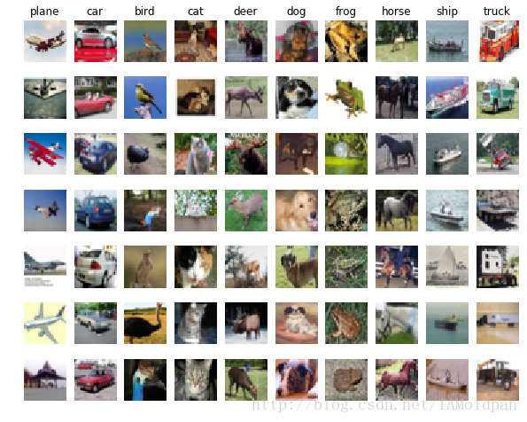
# create a small development set as a subset of the training data;
# we can use this for development so our code runs faster.
num_training = 49000
num_validation = 1000
num_test = 1000
num_dev = 500

# Our validation set will be num_validation points from the original
# training set.
mask = range(num_training, num_training + num_validation)
X_val = X_train[mask]
y_val = y_train[mask]

# Our training set will be the first num_train points from the original
# training set.
mask = range(num_training)
X_train = X_train[mask]
y_train = y_train[mask]

# We will also make a development set, which is a small subset of
# the training set.
mask = np.random.choice(num_training, num_dev, replace=False)
X_dev = X_train[mask]
y_dev = y_train[mask]

# We use the first num_test points of the original test set as our
# test set.
mask = range(num_test)
X_test = X_test[mask]
y_test = y_test[mask]

print('Train data shape: ', X_train.shape)
print('Train labels shape: ', y_train.shape)
print('Validation data shape: ', X_val.shape)
print('Validation labels shape: ', y_val.shape)
print('Test data shape: ', X_test.shape)
print('Test labels shape: ', y_test.shape)
Train data shape: (49000, 32, 32, 3)
Train labels shape: (49000,)
Validation data shape: (1000, 32, 32, 3)
Validation labels shape: (1000,)
Test data shape: (1000, 32, 32, 3)
Test labels shape: (1000,)
# 预处理: 将图像数据转化为一行
X_train = np.reshape(X_train, (X_train.shape[0], -1))
X_val = np.reshape(X_val, (X_val.shape[0], -1))
X_test = np.reshape(X_test, (X_test.shape[0], -1))
X_dev = np.reshape(X_dev, (X_dev.shape[0], -1))

# 为了确保操作正确,打印出来转换后的值
print('Training data shape: ', X_train.shape)
print('Validation data shape: ', X_val.shape)
print('Test data shape: ', X_test.shape)
print('dev data shape: ', X_dev.shape)
Training data shape: (49000, 3072)
Validation data shape: (1000, 3072)
Test data shape: (1000, 3072)
dev data shape: (500, 3072)
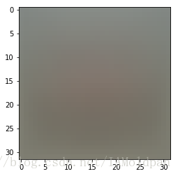
# 预处理: 减去均值图像
# 首先: 计算训练集图像中的均值
mean_image = np.mean(X_train, axis=0)
print(mean_image[:10]) # print a few of the elements
plt.figure(figsize=(4,4))
plt.imshow(mean_image.reshape((32,32,3)).astype('uint8')) # 将均值图像可视化
plt.show()
[ 130.64189796 135.98173469 132.47391837 130.05569388 135.34804082
131.75402041 130.96055102 136.14328571 132.47636735 131.48467347]
# 其次: 训练集和测试集中的图像都减去均值图像
X_train -= mean_image
X_val -= mean_image
X_test -= mean_image
X_dev -= mean_image
# 最后: append the bias dimension of ones (i.e. bias trick) so that our SVM
# only has to worry about optimizing a single weight matrix W.
X_train = np.hstack([X_train, np.ones((X_train.shape[0], 1))])
X_val = np.hstack([X_val, np.ones((X_val.shape[0], 1))])
X_test = np.hstack([X_test, np.ones((X_test.shape[0], 1))])
X_dev = np.hstack([X_dev, np.ones((X_dev.shape[0], 1))])
print(X_train.shape, X_val.shape, X_test.shape, X_dev.shape)(49000, 3073) (1000, 3073) (1000, 3073) (500, 3073)
# Evaluate the naive implementation of the loss we provided for you:
from cs231n.classifiers.linear_svm import svm_loss_naive
import time

# generate a random SVM weight matrix of small numbers
W = np.random.randn(3073, 10) * 0.0001

loss, grad = svm_loss_naive(W, X_dev, y_dev, 0.000005)
print('loss: %f' % (loss, ))
loss: 8.725495
# Once you've implemented the gradient, recompute it with the code below
# and gradient check it with the function we provided for you

# Compute the loss and its gradient at W.
loss, grad = svm_loss_naive(W, X_dev, y_dev, 0.0)

# Numerically compute the gradient along several randomly chosen dimensions, and
# compare them with your analytically computed gradient. The numbers should match
# almost exactly along all dimensions.
from cs231n.gradient_check import grad_check_sparse
f = lambda w: svm_loss_naive(w, X_dev, y_dev, 0.0)[0]
grad_numerical = grad_check_sparse(f, W, grad)

# do the gradient check once again with regularization turned on
# you didn't forget the regularization gradient did you?
loss, grad = svm_loss_naive(W, X_dev, y_dev, 5e1)
f = lambda w: svm_loss_naive(w, X_dev, y_dev, 5e1)[0]
grad_numerical = grad_check_sparse(f, W, grad)
numerical: -5.237454 analytic: -5.237454, relative error: 3.449639e-11
numerical: 6.266499 analytic: 6.266499, relative error: 2.319760e-11
numerical: 30.181612 analytic: 30.170690, relative error: 1.809656e-04
numerical: -0.804969 analytic: -0.804969, relative error: 2.856416e-12
numerical: -16.330168 analytic: -16.330168, relative error: 1.836775e-11
numerical: -13.194640 analytic: -13.194640, relative error: 2.749315e-11
numerical: -22.560453 analytic: -22.560453, relative error: 3.632089e-12
numerical: 7.740383 analytic: 7.740383, relative error: 9.546872e-13
numerical: 23.182039 analytic: 23.182039, relative error: 7.538815e-12
numerical: 20.514965 analytic: 20.514965, relative error: 8.834436e-12
numerical: 0.754403 analytic: 0.753503, relative error: 5.965723e-04
numerical: -2.838379 analytic: -2.837040, relative error: 2.358734e-04
numerical: 1.437758 analytic: 1.446441, relative error: 3.010690e-03
numerical: -50.392832 analytic: -50.395267, relative error: 2.415651e-05
numerical: -1.695855 analytic: -1.692918, relative error: 8.665519e-04
numerical: 10.391543 analytic: 10.391228, relative error: 1.512090e-05
numerical: 3.822426 analytic: 3.824819, relative error: 3.128660e-04
numerical: 9.237629 analytic: 9.233266, relative error: 2.362146e-04
numerical: 8.480450 analytic: 8.476681, relative error: 2.222481e-04
numerical: -10.077737 analytic: -10.074495, relative error: 1.608788e-04
# Next implement the function svm_loss_vectorized; for now only compute the loss;
# we will implement the gradient in a moment.
tic = time.time()
loss_naive, grad_naive = svm_loss_naive(W, X_dev, y_dev, 0.000005)
toc = time.time()
print('Naive loss: %e computed in %fs' % (loss_naive, toc - tic))

from cs231n.classifiers.linear_svm import svm_loss_vectorized
tic = time.time()
loss_vectorized, _ = svm_loss_vectorized(W, X_dev, y_dev, 0.000005)
toc = time.time()
print('Vectorized loss: %e computed in %fs' % (loss_vectorized, toc - tic))

# The losses should match but your vectorized implementation should be much faster.
print('difference: %f' % (loss_naive - loss_vectorized))
Naive loss: 8.725495e+00 computed in 0.105780s
Vectorized loss: 8.725495e+00 computed in 0.009526s
difference: 0.000000
# Complete the implementation of svm_loss_vectorized, and compute the gradient
# of the loss function in a vectorized way.

# The naive implementation and the vectorized implementation should match, but
# the vectorized version should still be much faster.
tic = time.time()
_, grad_naive = svm_loss_naive(W, X_dev, y_dev, 0.000005)
toc = time.time()
print('Naive loss and gradient: computed in %fs' % (toc - tic))

tic = time.time()
_, grad_vectorized = svm_loss_vectorized(W, X_dev, y_dev, 0.000005)
toc = time.time()
print('Vectorized loss and gradient: computed in %fs' % (toc - tic))

# The loss is a single number, so it is easy to compare the values computed
# by the two implementations. The gradient on the other hand is a matrix, so
# we use the Frobenius norm to compare them.
difference = np.linalg.norm(grad_naive - grad_vectorized, ord='fro')
print('difference: %f' % difference)
Naive loss and gradient: computed in 0.106282s
Vectorized loss and gradient: computed in 0.003010s
difference: 0.000000
# In the file linear_classifier.py, implement SGD in the function
# LinearClassifier.train() and then run it with the code below.
from cs231n.classifiers import LinearSVM
svm = LinearSVM()
tic = time.time()
loss_hist = svm.train(X_train, y_train, learning_rate=1e-7, reg=2.5e4,
                      num_iters=1500, verbose=True)
toc = time.time()
print('That took %fs' % (toc - tic))
iteration 0 / 1500: loss 404.022882
iteration 100 / 1500: loss 243.534573
iteration 200 / 1500: loss 148.575475
iteration 300 / 1500: loss 91.002578
iteration 400 / 1500: loss 57.258468
iteration 500 / 1500: loss 36.051044
iteration 600 / 1500: loss 23.728693
iteration 700 / 1500: loss 16.554524
iteration 800 / 1500: loss 11.944083
iteration 900 / 1500: loss 9.118885
iteration 1000 / 1500: loss 7.359942
iteration 1100 / 1500: loss 6.902793
iteration 1200 / 1500: loss 6.010290
iteration 1300 / 1500: loss 5.055070
iteration 1400 / 1500: loss 5.107912
That took 8.513293s
# A useful debugging strategy is to plot the loss as a function of
# iteration number:
plt.plot(loss_hist)
plt.xlabel('Iteration number')
plt.ylabel('Loss value')
plt.show()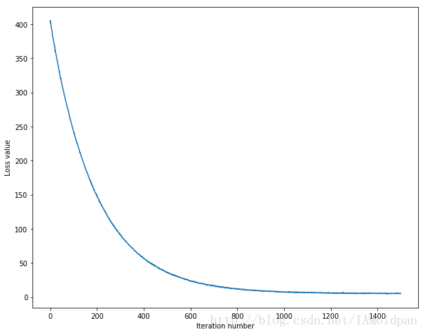
# Write the LinearSVM.predict function and evaluate the performance on both the
# training and validation set
y_train_pred = svm.predict(X_train)
print('training accuracy: %f' % (np.mean(y_train == y_train_pred), ))
y_val_pred = svm.predict(X_val)
print('validation accuracy: %f' % (np.mean(y_val == y_val_pred), ))
training accuracy: 0.383592
validation accuracy: 0.382000
# Use the validation set to tune hyperparameters (regularization strength and
# learning rate). You should experiment with different ranges for the learning
# rates and regularization strengths; if you are careful you should be able to
# get a classification accuracy of about 0.4 on the validation set.
# 使用验证集去调整超参数(正则化参数和学习率)。你应该测试不同的超参数,如果足够
# 仔细,你可以得到大概40%的正确率
learning_rates = [1.4e-7, 1.5e-7, 1.6e-7]
regularization_strengths = [(1+i*0.1)*1e4 for i in range(-3,3)] + [(2+0.1*i)*1e4 for i in range(-3,3)]

# results is dictionary mapping tuples of the form
# (learning_rate, regularization_strength) to tuples of the form
# (training_accuracy, validation_accuracy). The accuracy is simply the fraction
# of data points that are correctly classified.
# 结果是一个字典{(学习率, 正则化参数):(训练集准确度,验证集准确度)}
results = {}
best_val = -1   # 目前为止最高验证集的准确度
best_svm = None # LinearSVM 对象所能达到最高的正确度

################################################################################
# TODO:                                                                        #
# Write code that chooses the best hyperparameters by tuning on the validation #
# set. For each combination of hyperparameters, train a linear SVM on the      #
# training set, compute its accuracy on the training and validation sets, and  #
# store these numbers in the results dictionary. In addition, store the best   #
# validation accuracy in best_val and the LinearSVM object that achieves this  #
# accuracy in best_svm.                                                        #
#                                                                              #
# Hint: You should use a small value for num_iters as you develop your         #
# validation code so that the SVMs don't take much time to train; once you are #
# confident that your validation code works, you should rerun the validation   #
# code with a larger value for num_iters.                                      #
################################################################################
for rs in regularization_strengths:
    for lr in learning_rates:
        svm = LinearSVM()
        loss_hist = svm.train(X_train, y_train, lr, rs, num_iters=3000)
        y_train_pred = svm.predict(X_train)
        train_accuracy = np.mean(y_train == y_train_pred)
        y_val_pred = svm.predict(X_val)
        val_accuracy = np.mean(y_val == y_val_pred)
        if val_accuracy > best_val:
            best_val = val_accuracy
            best_svm = svm
        results[(lr,rs)] = train_accuracy, val_accuracy
################################################################################
#                              END OF YOUR CODE                                #
################################################################################

# Print out results.
for lr, reg in sorted(results):
    train_accuracy, val_accuracy = results[(lr, reg)]
    print('lr %e reg %e train accuracy: %f val accuracy: %f' % (
                lr, reg, train_accuracy, val_accuracy))

print('best validation accuracy achieved during cross-validation: %f' % best_val)
lr 1.400000e-07 reg 7.000000e+03 train accuracy: 0.400694 val accuracy: 0.392000
lr 1.400000e-07 reg 8.000000e+03 train accuracy: 0.391980 val accuracy: 0.404000
lr 1.400000e-07 reg 9.000000e+03 train accuracy: 0.394612 val accuracy: 0.385000
lr 1.400000e-07 reg 1.000000e+04 train accuracy: 0.393735 val accuracy: 0.377000
lr 1.400000e-07 reg 1.100000e+04 train accuracy: 0.393163 val accuracy: 0.392000
lr 1.400000e-07 reg 1.200000e+04 train accuracy: 0.390082 val accuracy: 0.381000
lr 1.400000e-07 reg 1.700000e+04 train accuracy: 0.389449 val accuracy: 0.389000
lr 1.400000e-07 reg 1.800000e+04 train accuracy: 0.385204 val accuracy: 0.390000
lr 1.400000e-07 reg 1.900000e+04 train accuracy: 0.380367 val accuracy: 0.387000
lr 1.400000e-07 reg 2.000000e+04 train accuracy: 0.383816 val accuracy: 0.394000
lr 1.400000e-07 reg 2.100000e+04 train accuracy: 0.385347 val accuracy: 0.391000
lr 1.400000e-07 reg 2.200000e+04 train accuracy: 0.376571 val accuracy: 0.384000
lr 1.500000e-07 reg 7.000000e+03 train accuracy: 0.397082 val accuracy: 0.403000
lr 1.500000e-07 reg 8.000000e+03 train accuracy: 0.394082 val accuracy: 0.401000
lr 1.500000e-07 reg 9.000000e+03 train accuracy: 0.393878 val accuracy: 0.395000
lr 1.500000e-07 reg 1.000000e+04 train accuracy: 0.393265 val accuracy: 0.382000
lr 1.500000e-07 reg 1.100000e+04 train accuracy: 0.389429 val accuracy: 0.401000
lr 1.500000e-07 reg 1.200000e+04 train accuracy: 0.380653 val accuracy: 0.386000
lr 1.500000e-07 reg 1.700000e+04 train accuracy: 0.379714 val accuracy: 0.368000
lr 1.500000e-07 reg 1.800000e+04 train accuracy: 0.381918 val accuracy: 0.368000
lr 1.500000e-07 reg 1.900000e+04 train accuracy: 0.379143 val accuracy: 0.371000
lr 1.500000e-07 reg 2.000000e+04 train accuracy: 0.372184 val accuracy: 0.379000
lr 1.500000e-07 reg 2.100000e+04 train accuracy: 0.379367 val accuracy: 0.384000
lr 1.500000e-07 reg 2.200000e+04 train accuracy: 0.374184 val accuracy: 0.375000
lr 1.600000e-07 reg 7.000000e+03 train accuracy: 0.396408 val accuracy: 0.391000
lr 1.600000e-07 reg 8.000000e+03 train accuracy: 0.393245 val accuracy: 0.392000
lr 1.600000e-07 reg 9.000000e+03 train accuracy: 0.395224 val accuracy: 0.395000
lr 1.600000e-07 reg 1.000000e+04 train accuracy: 0.392939 val accuracy: 0.397000
lr 1.600000e-07 reg 1.100000e+04 train accuracy: 0.388000 val accuracy: 0.398000
lr 1.600000e-07 reg 1.200000e+04 train accuracy: 0.390163 val accuracy: 0.392000
lr 1.600000e-07 reg 1.700000e+04 train accuracy: 0.388980 val accuracy: 0.400000
lr 1.600000e-07 reg 1.800000e+04 train accuracy: 0.380571 val accuracy: 0.373000
lr 1.600000e-07 reg 1.900000e+04 train accuracy: 0.370694 val accuracy: 0.377000
lr 1.600000e-07 reg 2.000000e+04 train accuracy: 0.385041 val accuracy: 0.379000
lr 1.600000e-07 reg 2.100000e+04 train accuracy: 0.384939 val accuracy: 0.391000
lr 1.600000e-07 reg 2.200000e+04 train accuracy: 0.374327 val accuracy: 0.403000
best validation accuracy achieved during cross-validation: 0.404000
# Visualize the cross-validation results
import math
x_scatter = [math.log10(x[0]) for x in results]
y_scatter = [math.log10(x[1]) for x in results]

# plot training accuracy
marker_size = 100
colors = [results[x][0] for x in results]
plt.subplot(2, 1, 1)
plt.scatter(x_scatter, y_scatter, marker_size, c=colors)
plt.colorbar()
plt.xlabel('log learning rate')
plt.ylabel('log regularization strength')
plt.title('CIFAR-10 training accuracy')

# plot validation accuracy
colors = [results[x][1] for x in results] # default size of markers is 20
plt.subplot(2, 1, 2)
plt.scatter(x_scatter, y_scatter, marker_size, c=colors)
plt.colorbar()
plt.xlabel('log learning rate')
plt.ylabel('log regularization strength')
plt.title('CIFAR-10 validation accuracy')
plt.show()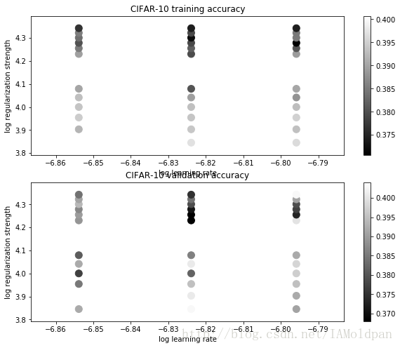
# Evaluate the best svm on test set
y_test_pred = best_svm.predict(X_test)
test_accuracy = np.mean(y_test == y_test_pred)
print('linear SVM on raw pixels final test set accuracy: %f' % test_accuracy)
linear SVM on raw pixels final test set accuracy: 0.384000
# 每个类中学习好的权重图片进行可视化
# 取决于你选择的学习率和正则化参数, 这些图可能不是特别好看
w = best_svm.W[:-1,:] # strip out the bias
w = w.reshape(32, 32, 3, 10)
w_min, w_max = np.min(w), np.max(w)
classes = ['plane', 'car', 'bird', 'cat', 'deer', 'dog', 'frog', 'horse', 'ship', 'truck']
for i in range(10):
    plt.subplot(2, 5, i + 1)

    # Rescale the weights to be between 0 and 255
    wimg = 255.0 * (w[:, :, :, i].squeeze() - w_min) / (w_max - w_min)
    plt.imshow(wimg.astype('uint8'))
    plt.axis('off')
    plt.title(classes[i])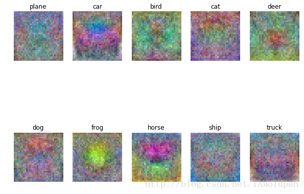
这些图像是权重系数转化而来的图,而分数是由权重系数和样本图像的内积得到的,如果想得到更高的分数,那么与之匹配的权重应该与样本尽可能相似。
linear_svm.py
import numpy as np
from random import shuffle
xrange = range


def svm_loss_naive(W, X, y, reg):
    """
    Structured SVM loss function, naive implementation (with loops).

    Inputs have dimension D, there are C classes, and we operate on minibatches
    of N examples.

    Inputs:
    - W: A numpy array of shape (D, C) containing weights.
    - X: A numpy array of shape (N, D) containing a minibatch of data.
    - y: A numpy array of shape (N,) containing training labels; y[i] = c means
        that X[i] has label c, where 0 <= c < C.
    - reg: (float) regularization strength

    Returns a tuple of:
    - loss as single float
    - gradient with respect to weights W; an array of same shape as W
    """
    dW = np.zeros(W.shape)  # initialize the gradient as zero

    # compute the loss and the gradient
    num_classes = W.shape[1]   #10
    num_train = X.shape[0]     #500
    loss = 0.0
    for i in xrange(num_train):
        scores = X[i].dot(W)
        correct_class_score = scores[y[i]]
        for j in xrange(num_classes):
            if j == y[i]:
                continue
            margin = scores[j] - correct_class_score + 1  # note delta = 1
            if margin > 0:
                loss += margin
                dW[:, j] += X[i].T
                dW[:, y[i]] += -X[i].T

    # Right now the loss is a sum over all training examples, but we want it
    # to be an average instead so we divide by num_train.
    loss /= num_train
    dW /= num_train

    # 添加正则化.
    loss += reg * np.sum(W * W)
    dW += reg * W

    #############################################################################
    # TODO:                                                                     #
    # Compute the gradient of the loss function and store it dW.                #
    # Rather that first computing the loss and then computing the derivative,   #
    # it may be simpler to compute the derivative at the same time that the     #
    # loss is being computed. As a result you may need to modify some of the    #
    # code above to compute the gradient.                                       #
    #############################################################################

    return loss, dW


def svm_loss_vectorized(W, X, y, reg):
    """
    Structured SVM loss function, vectorized implementation.

    Inputs and outputs are the same as svm_loss_naive.
    """
    loss = 0.0
    dW = np.zeros(W.shape)  # initialize the gradient as zero

    #############################################################################
    # TODO:                                                                     #
    # Implement a vectorized version of the structured SVM loss, storing the    #
    # result in loss.                                                           #
    #############################################################################
    num_train = X.shape[0]                   # 500
    num_classes = W.shape[1]                 # 10
    scores = X.dot(W)
    correct_class_scores = scores[range(num_train), list(y)].reshape(-1, 1)  #(N,1)
    margins = np.maximum(0, scores - correct_class_scores + 1)
    margins[range(num_train), list(y)] = 0
    loss = np.sum(margins) / num_train + 0.5 * reg * np.sum(W * W)

    #############################################################################
    #                             END OF YOUR CODE                              #
    #############################################################################

    #############################################################################
    # TODO:                                                                     #
    # Implement a vectorized version of the gradient for the structured SVM     #
    # loss, storing the result in dW.                                           #
    #                                                                           #
    # Hint: Instead of computing the gradient from scratch, it may be easier    #
    # to reuse some of the intermediate values that you used to compute the     #
    # loss.                                                                     #
    #############################################################################
    coeff_mat = np.zeros((num_train, num_classes))   #500 * 10
    coeff_mat[margins > 0] = 1
    coeff_mat[range(num_train), list(y)] = 0
    coeff_mat[range(num_train), list(y)] = -np.sum(coeff_mat, axis=1)

    dW = (X.T).dot(coeff_mat)
    dW = dW/num_train + reg * W
    #############################################################################
    #                             END OF YOUR CODE                              #
    #############################################################################

    return loss, dW
linear_classifier.py
from __future__ import print_function

import numpy as np
from cs231n.classifiers.linear_svm import *
from cs231n.classifiers.softmax import *

xrange = range


class LinearClassifier(object):

    def __init__(self):

        self.W = None

    def train(self, X, y, learning_rate=1e-3, reg=1e-5, num_iters=100,
            batch_size=200, verbose=False):
        """
        Train this linear classifier using stochastic gradient descent.

        Inputs:
        - X: A numpy array of shape (N, D) containing training data; there are N
          training samples each of dimension D.
        - y: A numpy array of shape (N,) containing training labels; y[i] = c
          means that X[i] has label 0 <= c < C for C classes.
        - learning_rate: (float) learning rate for optimization.
        - reg: (float) regularization strength.
        - num_iters: (integer) number of steps to take when optimizing
        - batch_size: (integer) number of training examples to use at each step.
        - verbose: (boolean) If true, print progress during optimization.

        Outputs:
        A list containing the value of the loss function at each training iteration.
        """
        num_train, dim = X.shape               # num_train:500  dim:3072
        num_classes = np.max(y) + 1            # 假设y取值0...k-1,其中k为y里面元素的数量
        if self.W is None:
            # lazily initialize W
            self.W = 0.001 * np.random.randn(dim, num_classes)

        # Run stochastic gradient descent to optimize W
        loss_history = []
        for it in xrange(num_iters):
            X_batch = None
            y_batch = None

            #########################################################################
            # TODO:                                                                 #
            # Sample batch_size elements from the training data and their           #
            # corresponding labels to use in this round of gradient descent.        #
            # Store the data in X_batch and their corresponding labels in           #
            # y_batch; after sampling X_batch should have shape (dim, batch_size)   #
            # and y_batch should have shape (batch_size,)                           #
            #                                                                       #
            # Hint: Use np.random.choice to generate indices. Sampling with         #
            # replacement is faster than sampling without replacement.              #
            #########################################################################
            mask = np.random.choice(num_train, batch_size, replace=False)
            X_batch = X[mask]
            y_batch = y[mask]
            #########################################################################
            #                       END OF YOUR CODE                                #
            #########################################################################

            # evaluate loss and gradient
            loss, grad = self.loss(X_batch, y_batch, reg)
            loss_history.append(loss)

            # perform parameter update
            #########################################################################
            # TODO:                                                                 #
            # Update the weights using the gradient and the learning rate.          #
            #########################################################################

            self.W += -learning_rate*grad

            #########################################################################
            #                       END OF YOUR CODE                                #
            #########################################################################

            if verbose and it % 100 == 0:
                print('iteration %d / %d: loss %f' % (it, num_iters, loss))

        return loss_history

    def predict(self, X):
        """
        Use the trained weights of this linear classifier to predict labels for
        data points.

        Inputs:
        - X: A numpy array of shape (N, D) containing training data; there are N
          training samples each of dimension D.

        Returns:
        - y_pred: Predicted labels for the data in X. y_pred is a 1-dimensional
          array of length N, and each element is an integer giving the predicted
          class.
        """
        y_pred = np.zeros(X.shape[0])
        ###########################################################################
        # TODO:                                                                   #
        # Implement this method. Store the predicted labels in y_pred.            #
        ###########################################################################
        scores = X.dot(self.W)
        y_pred = np.argmax(scores, axis=1)
        ###########################################################################
        #                           END OF YOUR CODE                              #
        ###########################################################################
        return y_pred

    def loss(self, X_batch, y_batch, reg):
        """
        Compute the loss function and its derivative.
        Subclasses will override this.

        Inputs:
        - X_batch: A numpy array of shape (N, D) containing a minibatch of N
          data points; each point has dimension D.
        - y_batch: A numpy array of shape (N,) containing labels for the minibatch.
        - reg: (float) regularization strength.

        Returns: A tuple containing:
        - loss as a single float
        - gradient with respect to self.W; an array of the same shape as W
        """
        pass


class LinearSVM(LinearClassifier):
    """ A subclass that uses the Multiclass SVM loss function """

    def loss(self, X_batch, y_batch, reg):
        return svm_loss_vectorized(self.W, X_batch, y_batch, reg)


class Softmax(LinearClassifier):
    """ A subclass that uses the Softmax + Cross-entropy loss function """

    def loss(self, X_batch, y_batch, reg):
      return softmax_loss_vectorized(self.W, X_batch, y_batch, reg)