2.Ransac是一种非常简单的算法
用于在一群样本中去掉噪声样本,得到有效的样本
采用随机抽样验证的方法,以下节选自wikipedia,选有用的贴了过来
RANSAC
RANSAC is an abbreviation for "RANdom SAmple Consensus". It is an algorithm to estimate parameters
of a mathematical model from a set of observed data which contains outliers . The algorithm was first
published by Fischler and Bolles in 1981.
A basic assumption is that the data consists of "inliers", i.e., data
points which can be explained by some set of model parameters, and
"outliers" which are data points that do not fit the model. In addition
to this, the data points can be subject to noise. The outliers can
come, e.g., from extreme values of the noise or from erroneous
measurements or incorrect hypotheses about the interpretation of data.
RANSAC also assumes that, given a (usually small) set of inliers, there
exists a procedure which can estimate the parameters of a model that
optimally explains or fits this data.
Example
A
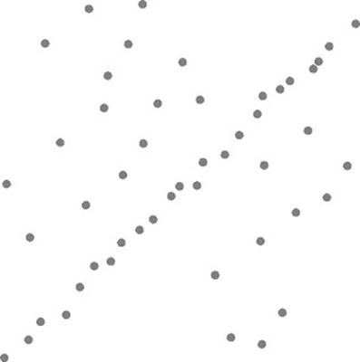
simple example is fitting of a 2D line to set of observations. Assuming
that this set contains both inliers, i.e., points which approximately
can be fitted to a line, and outliers, points which cannot be fitted to
this line, a simple least squares method for line fitting will in
general produce a line with a bad fit to the inliers. The reason is
that it is optimally fitted to all points, including the outliers.
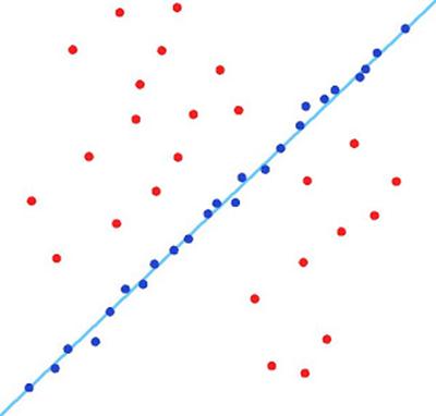
RANSAC, on the other hand, can produce a model which is only computed
from the inliers, provided that the probability of choosing only
inliers in the selection of data points is sufficiently high. There is
no guarantee for this situation, however, and there are a number of
algorithm parameters which must be carefully chosen to keep the level
of probability reasonably high.
Overview
The
input to the RANSAC algorithm is a set of observed data values, a
parameterized model which can explain or be fitted to the observations,
and some confidence parameters.
RANSAC achieves its goal by
iteratively selecting a random subset of the original data points.
These points are hypothetical inliers and this hypothesis is then
tested as follows. A model is fitted to the hypothetical inliers, that
is, all free parameters of the model are reconstructed from the point
set. All other data points are then tested against the fitted model,
that is, for every point of the remaining set, the algorithm determines
how well the point fits to the estimated model. If it fits well, that
point is also considered as a hypothetical inlier. If sufficiently many
points have been classified as hypothetical inliers relative to the
estimated model, then we have a model which is reasonably good.
However, it has only been estimated from the initial set of
hypothetical inliers, so we reestimate the model from the entire set of
point's hypothetical inliers. At the same time, we also estimate the
error of the inliers relative to the model.
This procedure is then
repeated a fixed number of times, each time producing either a model
which is rejected because too few points are classified as inliers or a
refined model together with a corresponding error measure. In the
latter case, we keep the refined model if its error is lower than the
last saved model.
Algorithm
The generic RANSAC algorithm works as follows:
input:
data - a set of observed data points
model - a model that can be fitted to data points
n - the minimum number of data values required to fit the model
k - the maximum number of iterations allowed in the algorithm
t - a threshold value for determining when a data point fits a model
d - the number of close data values required to assert that a model fits well to data
output:
bestfit - model parameters which best fit the data (or nil if no good model is found)
iterations := 0
bestfit := nil
besterr := infinity
while iterations <> d
(this implies that we may have found a good model now test
how good it is)
bettermodel := model parameters fitted to all points in maybeinliers and alsoinliers
thiserr := a measure of how well model fits these points
if thiserr <>
increment iterations
return bestfit
While
the parameter values of t and d have to be calculated from the
individual requirements it can be experimentally determined. The
interesting parameter of the RANSAC algorithm is k.
To calculate the
parameter k given the known probability w of a good data value, the
probability z of seeing only bad data values is used:
which leads to
To
gain additional confidence, the standard deviation or multiples thereof
can be added to k. The standard deviation of k is defined as
A
common case is that w is not well known beforehand, but some rough
value can be given. If n data values are given, the probability of
success is wn.
Advantages and disadvantages
An advantage
of RANSAC is its ability to do robust estimation of the model
parameters, i.e., it can estimate the parameters with a high degree of
accuracy even when outliers are present in the data set. A disadvantage
of RANSAC is that there is no upper bound on the time it takes to
compute these parameters. If an upper time bound is used, the solution
obtained may not be the most optimal one.
RANSAC can only estimate
one model for a particular data set. As for any one-model approach when
more two (or more) models exist, RANSAC may fail to find either one.
Applications
The
RANSAC algorithm is often used in computer vision, e.g., to
simultaneously solve the correspondence problem and estimate the
fundamental matrix related to a pair of stereo cameras.
References
M.
A. Fischler and R. C. Bolles (June 1981). "Random Sample Consensus: A
Paradigm for Model Fitting with Applications to Image Analysis and
Automated Cartography". Comm. of the ACM 24: 381--395.
doi:10.1145/358669.358692.
David A. Forsyth and Jean Ponce (2003). Computer Vision, a modern approach. Prentice Hall. ISBN ISBN 0-13-085198-1.
Richard
Hartley and Andrew Zisserman (2003). Multiple View Geometry in Computer
Vision, 2nd edition, Cambridge University Press.
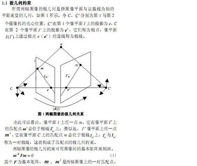
3.基础矩阵的概念:
基础矩阵把左边图像的一个点的图像坐标与它右边图像中的对应点的图像联系起来,他是一个3x3的退化矩阵,描述了两个立体图像对的外极限几何关系,其计算依赖于在两个图像中相对应的一组点。
#include <iostream>
#include <cv.h>
#include <highgui.h>
//------------ 各種外部変数 ----------//
double first[12][2] =
{
{488.362, 169.911},
{449.488, 174.44},
{408.565, 179.669},
{364.512, 184.56},
{491.483, 122.366},
{451.512, 126.56},
{409.502, 130.342},
{365.5, 134},
{494.335, 74.544},
{453.5, 76.5},
{411.646, 79.5901},
{366.498, 81.6577}
};
double second[12][2] =
{
{526.605, 213.332},
{470.485, 207.632},
{417.5, 201},
{367.485, 195.632},
{530.673, 156.417},
{473.749, 151.39},
{419.503, 146.656},
{368.669, 142.565},
{534.632, 97.5152},
{475.84, 94.6777},
{421.16, 90.3223},
{368.5, 87.5}
};
//---- 支持功能 ---//
double GetYCoord(double x, double a,double b,double c)
{
return -(a*x+c)/b;
}
int main(int argc,char *argv[])
{
CvMat *firstM = cvCreateMat(12,2,CV_64FC1);
cvSetData(firstM,first,firstM->step);
CvMat *secondM = cvCreateMat(12,2,CV_64FC1);
cvSetData(secondM,second,secondM->step);
CvMat *FMat= cvCreateMat(3,3,CV_64FC1);
if(cvFindFundamentalMat(firstM,secondM,FMat,CV_FM_RANSAC,1.00,0.99) == 0){ //获取基础矩阵F
std::cerr << "Can't Get F Mat/n";
return -1;
}
CvMat *lines = cvCreateMat(12,3,CV_64FC1);
cvComputeCorrespondEpilines(firstM,1,FMat,lines); //绘制外极线
IplImage *imgB = cvLoadImage( "second.png", CV_LOAD_IMAGE_ANYDEPTH | CV_LOAD_IMAGE_ANYCOLOR);
IplImage *imgA = cvLoadImage( "first.png", CV_LOAD_IMAGE_ANYDEPTH | CV_LOAD_IMAGE_ANYCOLOR);
if(imgB == NULL || imgA == NULL){
std::cout<<"Can't Load Image ./n";
return -1;
}
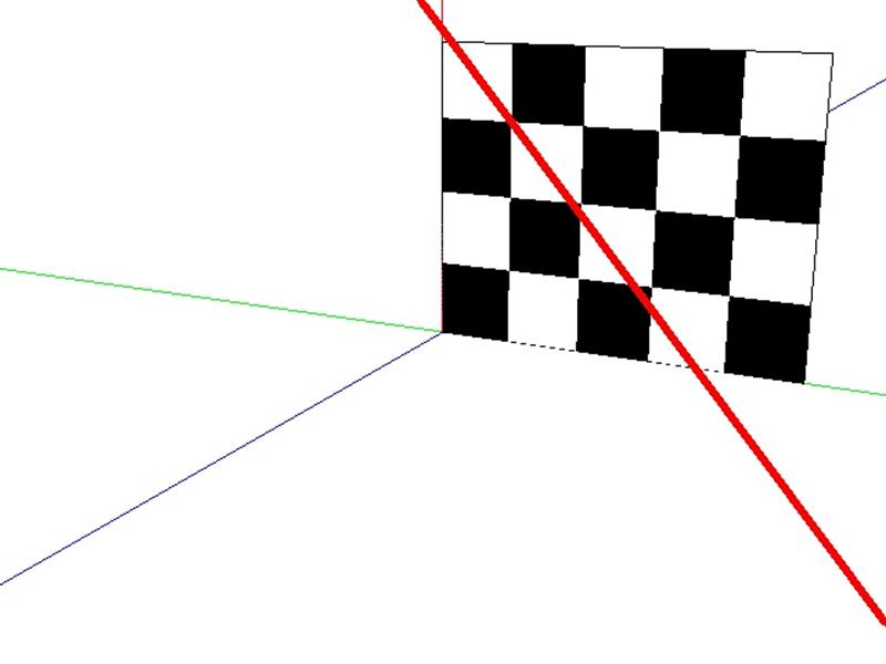
//绘制外极线
cvLine(imgB,
cvPoint( //始点
0, // x
cvRound(// y
GetYCoord(0,CV_MAT_ELEM(*lines,double,11,0),
CV_MAT_ELEM(*lines,double,11,1),CV_MAT_ELEM(*lines,double,11,2)))
),
cvPoint( //終点
imgB->width,// x
cvRound( // y
GetYCoord(imgB->width,CV_MAT_ELEM(*lines,double,11,0),
CV_MAT_ELEM(*lines,double,11,1),
CV_MAT_ELEM(*lines,double,11,2)))
),
CV_RGB(255,0,0),5);
//提请第三点
cvDrawRect(imgA,
cvPoint(cvRound(CV_MAT_ELEM(*firstM,double,11,0)),cvRound(CV_MAT_ELEM(*firstM,double,11,1))),
cvPoint(cvRound(CV_MAT_ELEM(*firstM,double,11,0)),cvRound(CV_MAT_ELEM(*firstM,double,11,1))),
CV_RGB(0,255,0),
8);
cvNamedWindow("second",CV_WINDOW_AUTOSIZE);
cvShowImage("second",imgB);
cvNamedWindow("first",CV_WINDOW_AUTOSIZE);
cvShowImage("first",imgA);
cvReleaseMat(&firstM);
cvReleaseMat(&secondM);
cvReleaseMat(&FMat);
cvReleaseImage( &imgA );
cvReleaseImage( &imgB);
cvReleaseMat(&lines);
cvWaitKey(0);
cvDestroyAllWindows();
return EXIT_SUCCESS;
}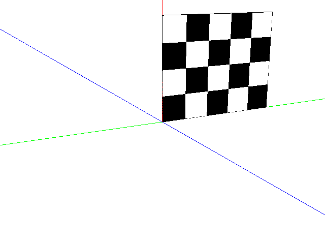
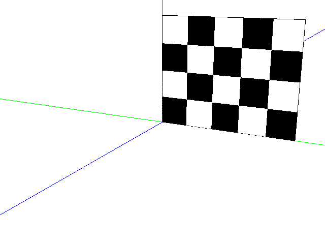
结果: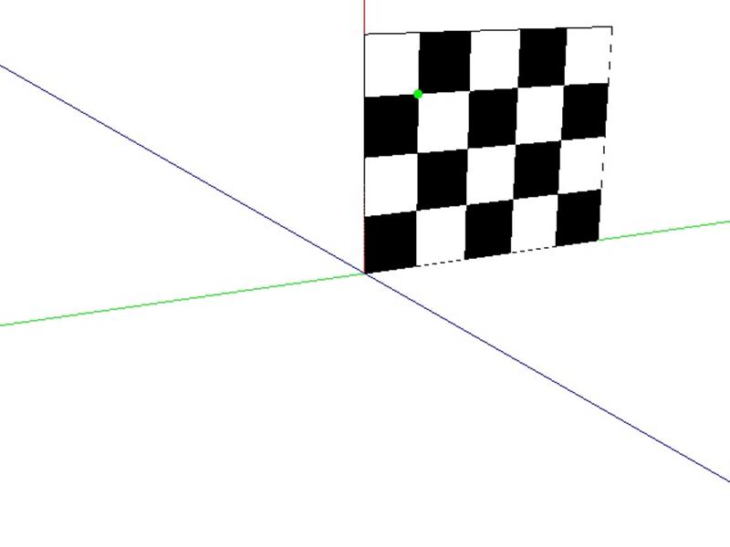
作者:gnuhpc
出处:http://www.cnblogs.com/gnuhpc/
除非另有声明,本网站采用知识共享“署名 2.5 中国大陆”许可协议授权。