
%%%% Tutorial on the basic structure of using a planar decision boundary
%%%% to divide a collection of data-points into two classes.
%%%% by Rajeev Raizada, Jan.2010
%%%%
%%%% Please mail any comments or suggestions to: raizada at cornell dot edu
%%%%
%%%% Probably the best way to look at this program is to read through it
%%%% line by line, and paste each line into the Matlab command window
%%%% in turn. That way, you can see what effect each individual command has.
%%%%
%%%% Alternatively, you can run the program directly by typing
%%%%
%%%% classification_plane_tutorial
%%%%
%%%% into your Matlab command window.
%%%% Do not type ".m" at the end
%%%% If you run the program all at once, all the Figure windows
%%%% will get made at once and will be sitting on top of each other.
%%%% You can move them around to see the ones that are hidden beneath.
%%%%%%%%%%%%%%%%%%%%%%%%%%%%%%%%%%%%%%%%%%%%%%%%%%%%%%%%%%%%%%%%%%%%%%%
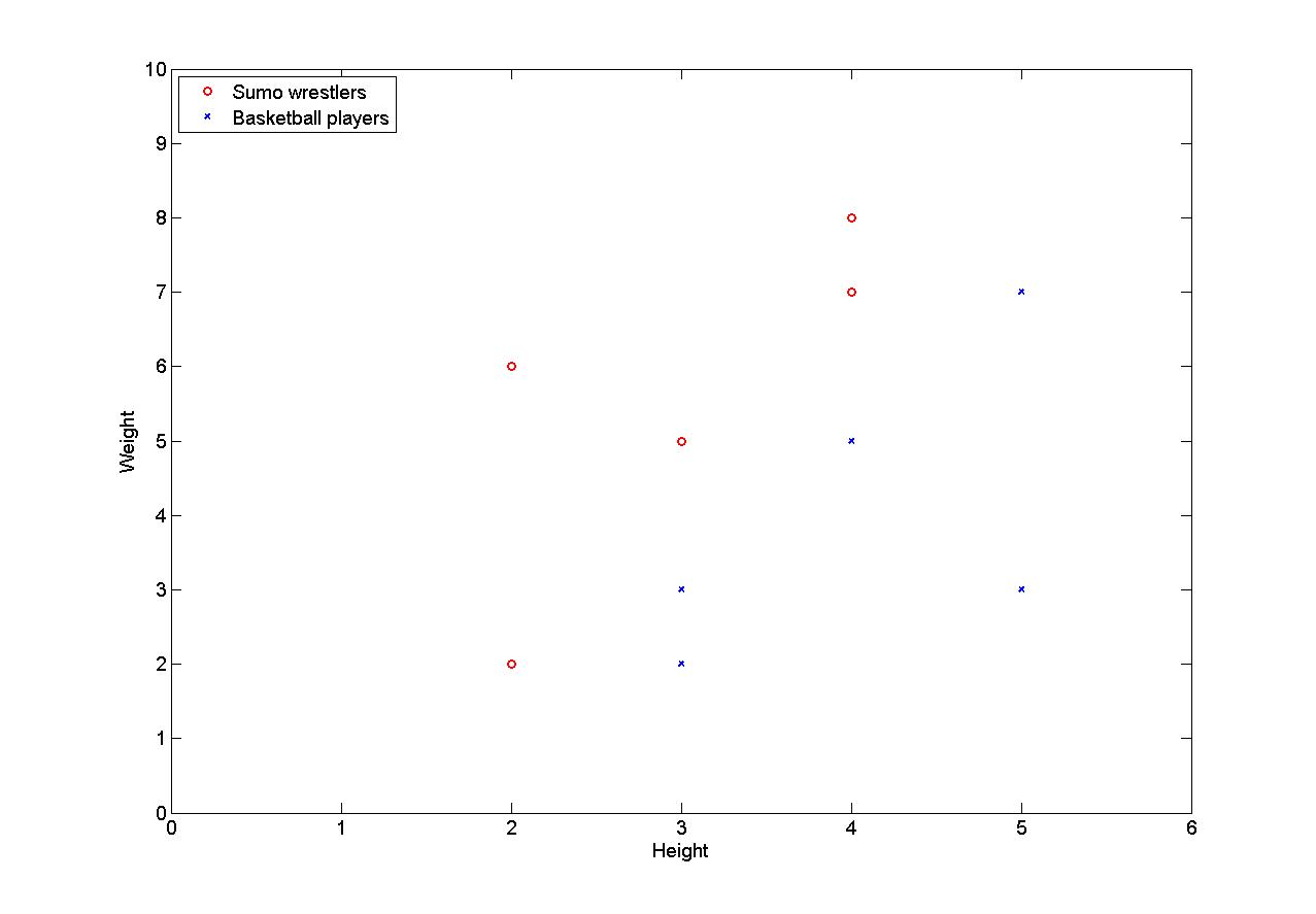
%%%% Let's look at a toy example: classifying people as either
%%%% sumo wrestlers or basketball players, depending on their height and weight.
%%%% Let's call the x-axis height and the y-axis weight
sumo_wrestlers = [ 4 8; ...
2 6; ...
2 2; ...
3 5; ...
4 7];
basketball_players = [ 3 2; ...
4 5; ...
5 3; ...
5 7; ...
3 3];
%%% Let's plot this
figure(1);
clf;
set(gca,'FontSize',14);
plot(sumo_wrestlers(:,1),sumo_wrestlers(:,2),'ro','LineWidth',2);
hold on;
plot(basketball_players(:,1),basketball_players(:,2),'bx','LineWidth',2);
axis([0 6 0 10]);
xlabel('Height');
ylabel('Weight');
legend('Sumo wrestlers','Basketball players',2); % The 2 at the end means
% put the legend in top-left corner
%%%% In order to be able to train a classifier on the input vectors,
%%%% we need to know what the desired output categories are for each one.
%%%% Let's set this to be +1 for sumo wrestlers, and -1 for basketball players
desired_output_sumo = [ 1; ... % sumo_wrestlers = [ 4 8; ...
1; ... % 2 6; ...
1; ... % 2 2; ...
1; ... % 3 5; ...
1 ]; % 4 7];
desired_output_basketball = [ -1; ... % basketball_players = [ 3 2; ...
-1; ... % 4 5; ...
-1; ... % 5 3; ...
-1; ... % 5 7; ...
-1 ]; % 3 3 ];
all_desired_output = [ desired_output_sumo; ...
desired_output_basketball ];
%%%%%% We want to find a linear decision boundary,
%%%%%% i.e. simply a straight line, such that all the data points
%%%%%% on one side of the line get classified as sumo wrestlers,
%%%%%% i.e. get mapped onto the desired output of +1,
%%%%%% and all the data points on the other side get classified
%%%%%% as basketball players, i.e. get mapped onto the desired output of -1.
%%%%%%
%%%%%% The equation for a straight line has this form:
%%%%%% weight_vector * data_coords - offset_from_origin = 0;
%%%%%%
%%%%%% We're not so interested for now in the offset_from_origin term,
%%%%%% so we can get rid of that by subtracting the mean from our data,
%%%%%% so that it is all centered around the origin.
%%%%%% Let's stack up the sumo data on top of the bastetball players data
all_data = [ sumo_wrestlers; ...
basketball_players ];
%%%%%% Now let's subtract the mean from the data,
%%%%%% so that it is all centered around the origin.
%%%%%% Each dimension (height and weight) has its own column.
mean_column_vals = mean(all_data);
%%%%%% To subtract the mean from each column in Matlab,
%%%%%% we need to make a matrix full of column-mean values
%%%%%% that is the same size as the whole data matrix.
matrix_of_mean_vals = ones(size(all_data,1),1) * mean_column_vals;
zero_meaned_data = all_data - matrix_of_mean_vals;
%%%% Now, having gotten rid of that annoying offset_from_origin term,
%%%% we want to find a weight vector which gives us the best solution
%%%% that we can find to this equation:
%%%% zero_meaned_data * weights = all_desired_output;
%%%% But, there is no such perfect set of weights.
%%%% We can only get a best fit, such that
%%%% zero_meaned_data * weights = all_desired_output + error
%%%% where the error term is as small as possible.
%%%%
%%%% Note that our equation
%%%% zero_meaned_data * weights = all_desired_output
%%%%
%%%% has exactly the same form as the equation
%%%% from the tutorial code in
%%%% http://www.dartmouth.edu/~raj/Matlab/fMRI/design_matrix_tutorial.m
%%%% which is:
%%%% Design matrix * sensitivity vector = Voxel response
%%%%
%%%% The way we solve the equation is exactly the same, too.
%%%% If we could find a matrix-inverse of the data matrix,
%%%% then we could pre-multiply both sides by that inverse,
%%%% and that would give us the weights:
%%%%
%%%% inv(zero_meaned_data) * zero_meaned_data * weights = inv(zero_meaned_data) * all_desired_output
%%%% The inv(zero_meaned_data) and zero_meaned_data terms on the left
%%%% would cancel each other out, and we would be left with:
%%%% weights = inv(zero_meaned_data) * all_desired_output
%%%%
%%%% However, unfortunately there will in general not exist any
%%%% matrix-inverse of the data matrix zero_meaned_data.
%%%% Only square matrices have inverses, and not even all of them do.
%%%% Luckily, however, we can use something that plays a similar role,
%%%% called a pseudo-inverse. In Matlab, this is given by the command pinv.
%%%% The pseudo-inverse won't give us a perfect solution to the equation
%%%% zero_meaned_data * weights = all_desired_output
%%%% but it will give us the best approximate solution, which is what we want.
%%%%
%%%% So, instead of
%%%% weights = inv(zero_meaned_data) * all_desired_output
%%%% we have this equation:
weights = pinv(zero_meaned_data) * all_desired_output;
%%%% Let's have a look at how these weights carve up the input space
%%%% A useful Matlab command for making grids of points
%%%% which span a particular 2D space is called "meshgrid"
[input_space_X, input_space_Y] = meshgrid([-3:0.3:3],[-3:0.3:3]);
weighted_output_Z = input_space_X*weights(1) + input_space_Y*weights(2);
%%%% The weighted output gets turned into the category-decision +1
%%%% if it is greater than 0, and -1 if it is less than zero.
%%%% The easiest way to map positive numbers to +1
%%%% and negative numbers to -1
%%%% is by first mapping them to 1 and 0
%%%% by the inequality-test(weighted_output_Z>0)
%%%% and then turning 1 and 0 into +1 and -1
%%%% by multipling by 2 and subtracting 1.
decision_output_Z = 2*(weighted_output_Z>0) - 1;
figure(2);
clf;
hold on;
surf(input_space_X,input_space_Y,decision_output_Z);
%%% Let's show this decision surface in gray, from a good angle
colormap gray;
caxis([-3 3]); %%% Sets white and black values to +/-3, so +/-1 are gray
shading interp; %%% Makes the shading look prettier
grid on;
view(-10,60);
rotate3d on; %%% Make it so we can use mouse to rotate the 3d figure
set(gca,'FontSize',14);
title('Click and drag to rotate view');
%%%% Let's plot the zero-meaned sumo and basketball data on top of this
%%%% Each class has 5 members, in this case, so we'll subtract
%%%% a mean-column-values matrix with 5 rows, to make the matrix sizes match.
one_class_matrix_of_mean_vals = ones(5,1) * mean_column_vals;
zero_meaned_sumo_wrestlers = sumo_wrestlers - one_class_matrix_of_mean_vals;
zero_meaned_basketball_players = basketball_players - one_class_matrix_of_mean_vals;
plot3(zero_meaned_sumo_wrestlers(:,1),zero_meaned_sumo_wrestlers(:,2), ...
desired_output_sumo,'ro','LineWidth',5);
hold on;
plot3(zero_meaned_basketball_players(:,1),zero_meaned_basketball_players(:,2), ...
desired_output_basketball,'bx','LineWidth',5,'MarkerSize',15);
xlabel('Height');
ylabel('Weight');
zlabel('Classifier output');
分类前:
分类后:

本文转自二郎三郎博客园博客,原文链接:http://www.cnblogs.com/haore147/p/3606042.html,如需转载请自行联系原作者
