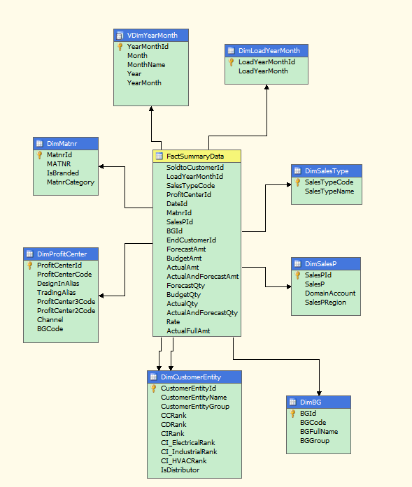
Normally, we have created a table, view in database or cube in SSAS, user can use Excel as a BI tool to display data. Here we have an Actual, Budget and Forecast data cube in SSAS.
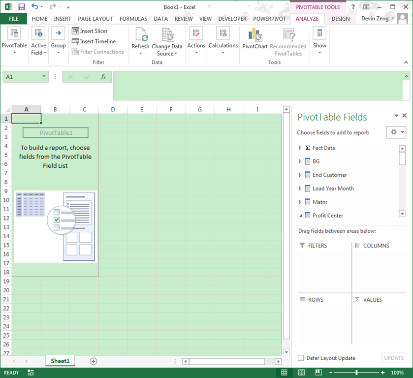
Open Excel, click “Data”->”From Other Sources”->”From Analysis Service” on Rabin menu, input SSAS server address, link to SSAS, select “PivotTable Report”, Excel will display cube dimensions and measures on the right panel.
Now, we can operate cube data in Excel now.
1. Columns Rows & Values
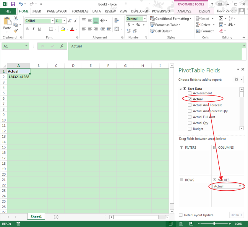
the first PivotTable Fields group is a measure group. Here “Fact Data” is our measure group. measure group fields only can be used in “Values”. For example, we want to our “Actual” data, drag “Actual” from field list to Values panel, Excel will display total actual data value on the left Excel cell like this:
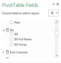
Except the measure group, other fields are dimension group. For example, we have a BG group in the fields list, expand this group we can see three fields:
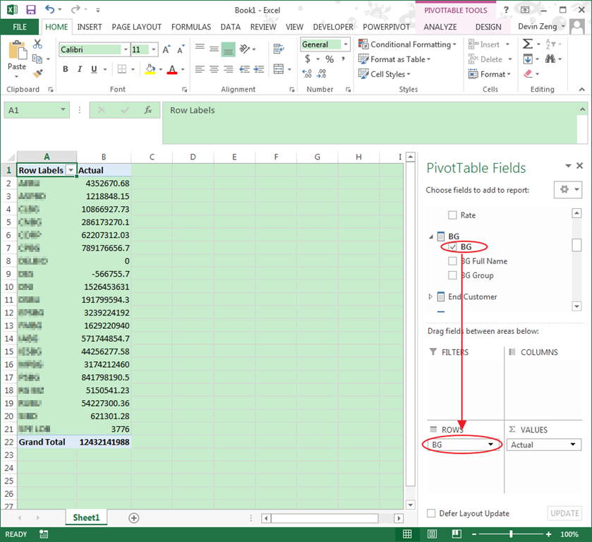
We can pick up our necessary fields and drag to “Columns “ panel or “Rows” panel. if we want display BG on left rows, drag BG to Rows panel, Excel will display every BG and Actual value on the left:
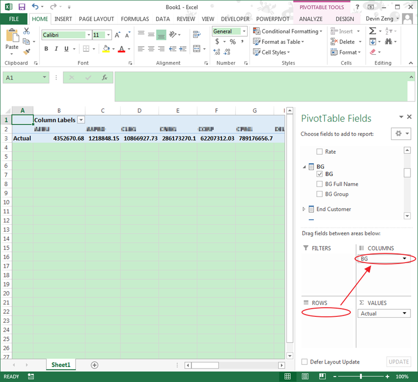
If you want to display BG on the top of every columns, just need drag “BG” from Rows panel to Columns panel. At the same time, left Excel region changed to BG column format:
If you don’t want display BG on Excel, you can drag the “BG” field from Columns panel to fields list or click “BG”, system will expand a menu, select “Remove Field”.
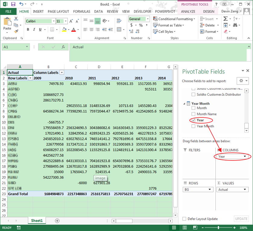
No, we want to see every year every BG actual value, we need drag BG to Rows panel, and find “Year Month” panel, drag “Year” to Columns panel, excel will display result table on the left:
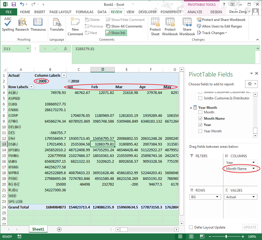
We can see there is a “Month Name” field in the Year Month dimension group, can we display every year every month BG actual value? Yes, just drag the “Month Name” to columns panel, under “Year” field, excel will refresh the excel, display month under year row, at the same time ,we can collect/expand Year node:
Use the same operation, we can add Profit Center, SalesP and other fields to excel rows or columns.
2. Filter
There is a Filters panel on the right, it is used to define which fields are filter and don’t need display in Excel.
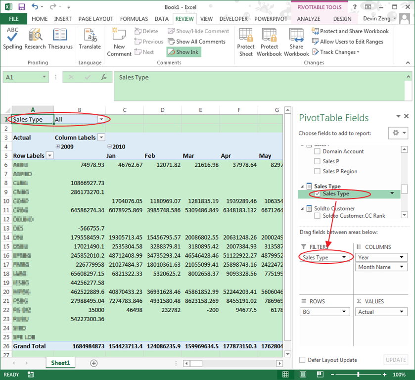
For example, we only want to display “Trading” actual data in the excel, we can find “Sales Type” and drag to Filters panel, excel will display filter control on the top left of the Excel and by default select “All”:
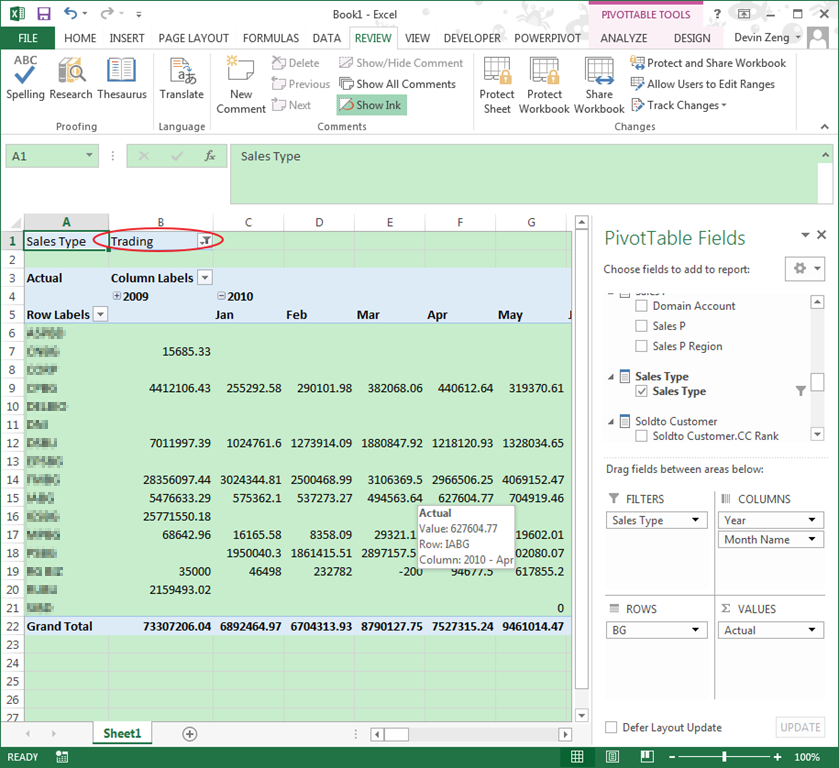
We just need “Trading” actual data, so select “Sales Type” equal “Trading”, we can see the Actual data table is refreshed:
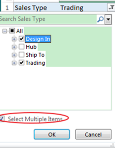
We also can select multiple values on the filter control, just only need select “Select Multiple Items” checkbox.
Filters panel only used to filter the hidden fields, that means filters never display on the main excel table. If you want to filter some fields and also need display them, we can use label filters.
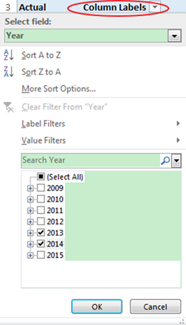
For example, we just need display 2013 and 2014 BG actual data, find the field in Columns panel or Rows panel. Year field is in columns panel, so click “Column Label”, excel will display a panel, remove all item select, just select 2013 and 2014 year:
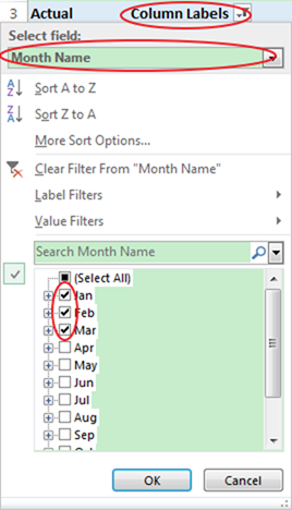
If we want to filter month field, also click “Column Labels”, at the panel, switch field to “Month Name”, the below items are refreshed. We just need display the first quarter actual data, so select the first three month:
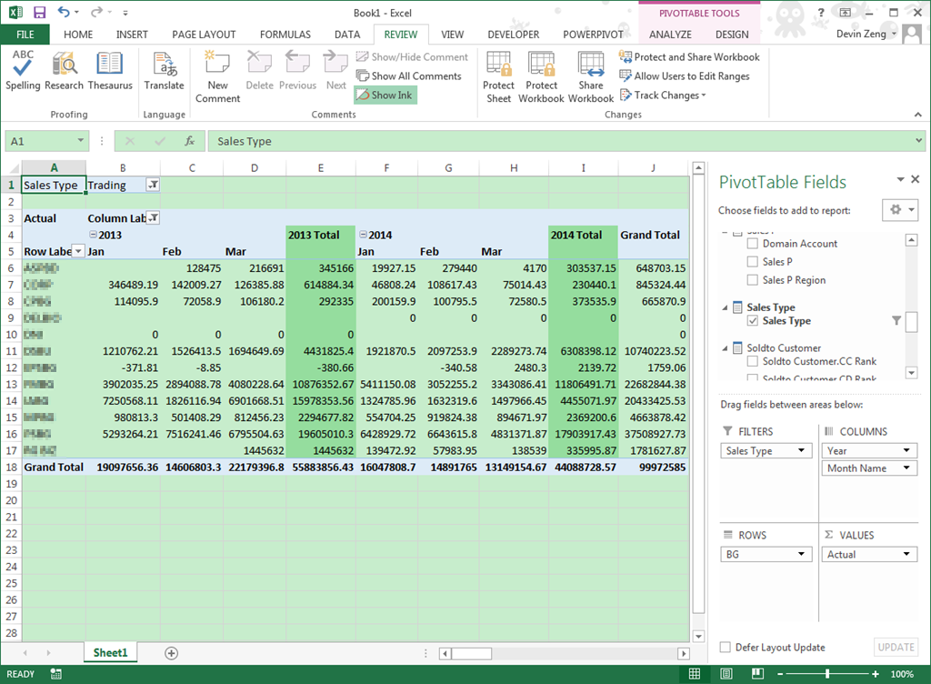
After all filter operation, excel will display 2013 2014 first quarter BG trading data:
3. Sort
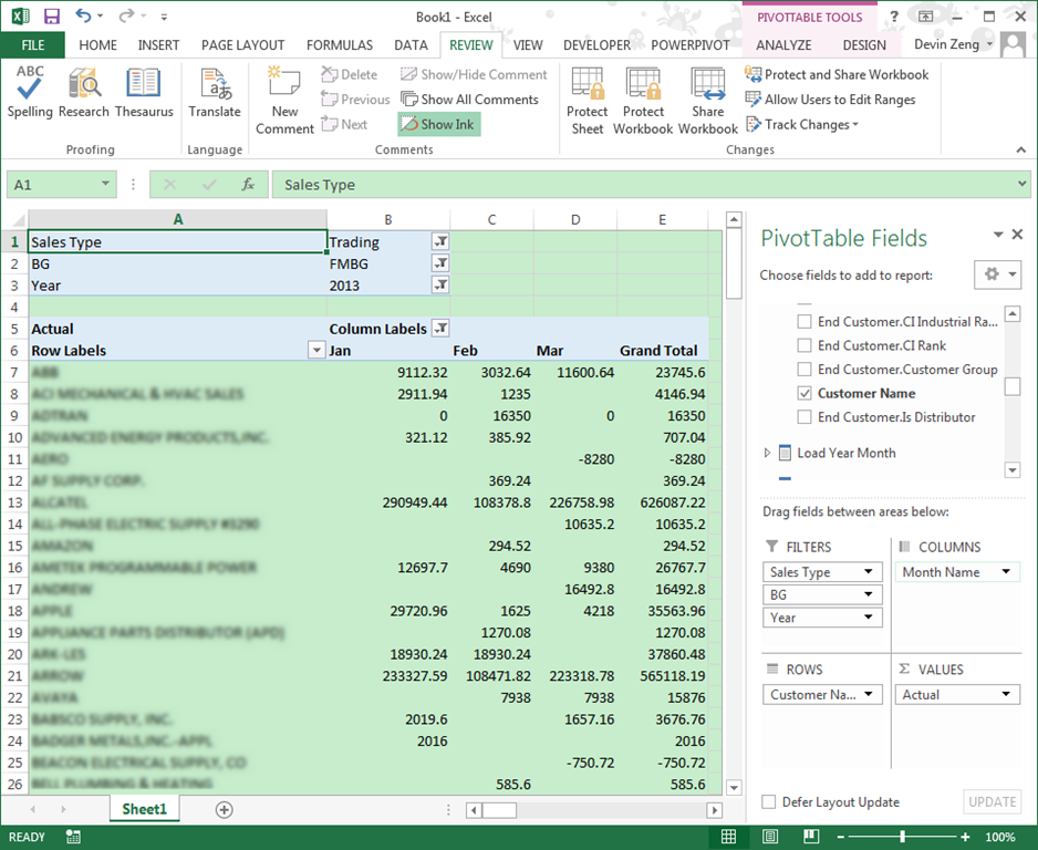
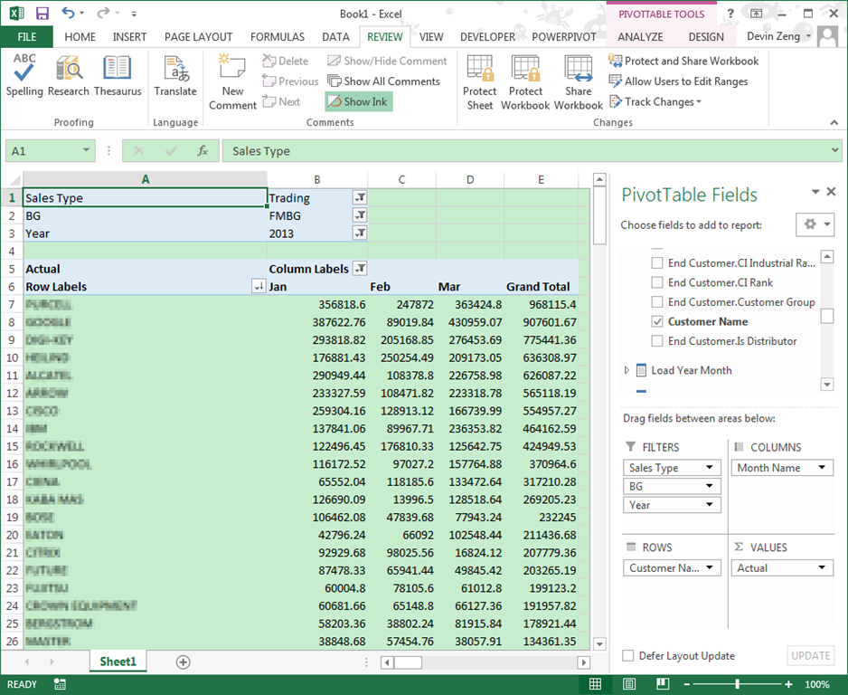
Sort function is only used to rows or columns. If we want to FMBG every customer 2013 first quarter trading data, we need adjust our excel fields and filter, after adjusted, excel display like below:
By default, customer sort by name alphabet, but usually we need sort them by actual value, we can follow these operations:
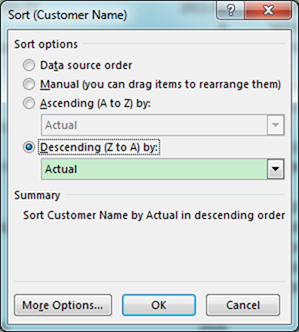
Click “Row Labels”, on the menu panel, select “More Sort Options”, excel will popup a Sort window. select “Descending by:” “Actual”:
Now, excel will display customer by their actual value:
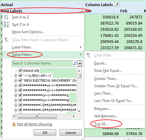
After sorted, we can use value filter to filter the customer list. If we just need top 20 customer, click “Row Labels”, on the popup panel, select “Value Filters”->”Top 10…”
Excel will open a Top 10 Filter window, input 20 and click OK.
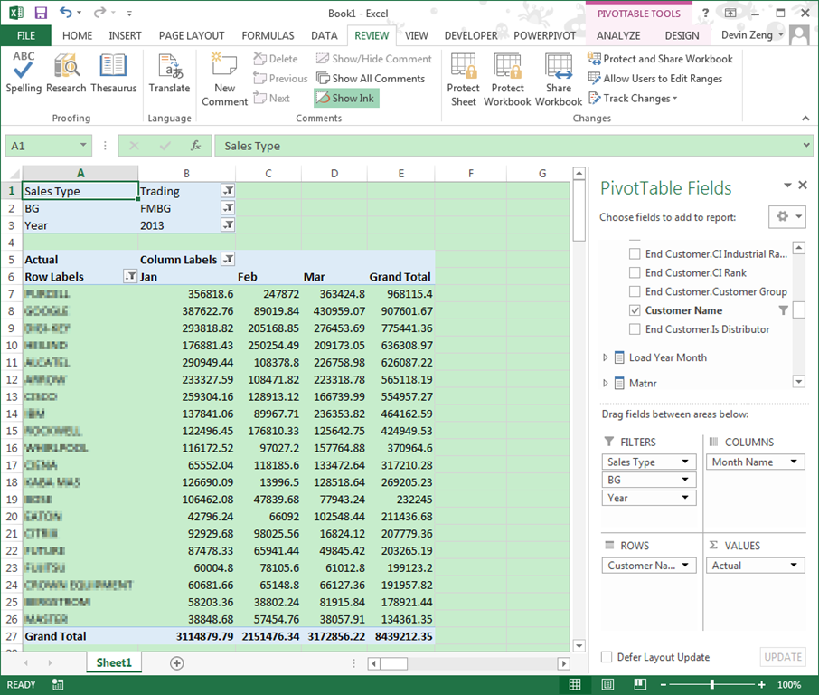
Excel will only display 20 customers, and the grand total value is these 20 customers sum value.
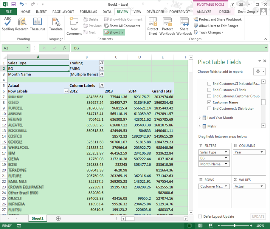
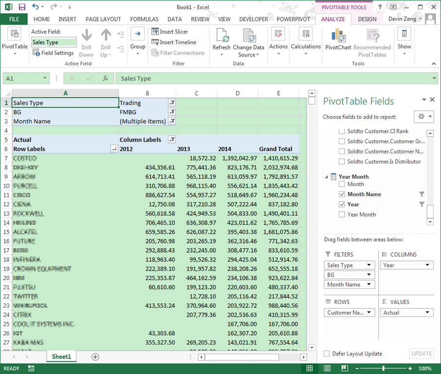
The sort value is grand total value, if there are 2012 to 2014 first quarter trading value in main table, and we just need sort by 2014 trading value, how to do it?
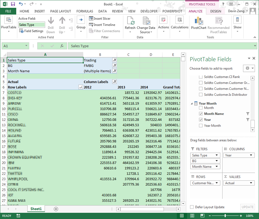
First we need adjust our excel fields, display 3 year data on columns:
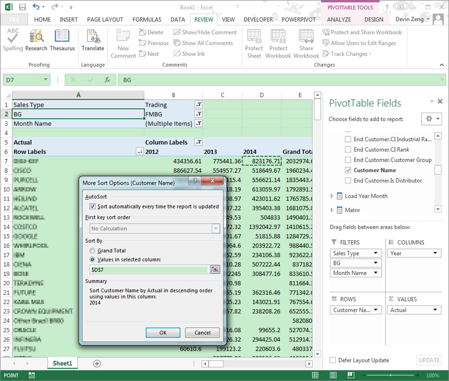
We can see our sort condition is 3 years total value. Now click “Row Labels”->”More Sort Options”, click “More Options”, system will open a More Sort Options window:
Select “Sort by Values in selected column”, and we just need sort by D column, so select any D column cell such as $D$7, and click OK. Excel will refresh and sort by D column values.
4. Format
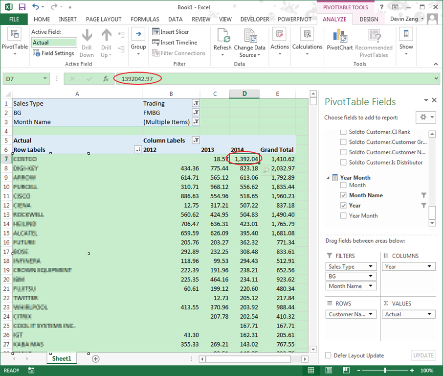
By default, excel doesn’t display 1000 separator and show 1~2 decimal place. We need change the format of number to a friendly format.
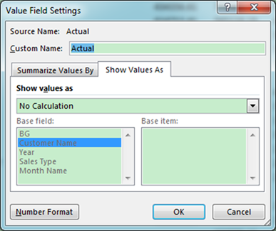
on the right bottom of Excel, click “Actual”, Excel will display a menu, select “Value Field Settings”, Excel will open a new window:
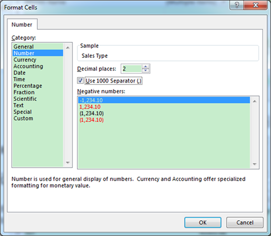
Click “Number Format” button, Excel will open a new window, select your favorite format:
Click “OK”, Excel refresh the main table, changed all “Actual” data format.
Some times, we need use “K”(thousand) as a basic unit, we can use custom format. Also the same operations, at last step, select Custom form, and input: “#,##0.00,”.
Now all actual values use “K” unit.
If we want to use “M”(million) as a basic unit, use custom format string: “#,##0.00,,”.
5. Total&Subtotal
By default, Excel will display row total and column total, at each sub fields show subtotal value.
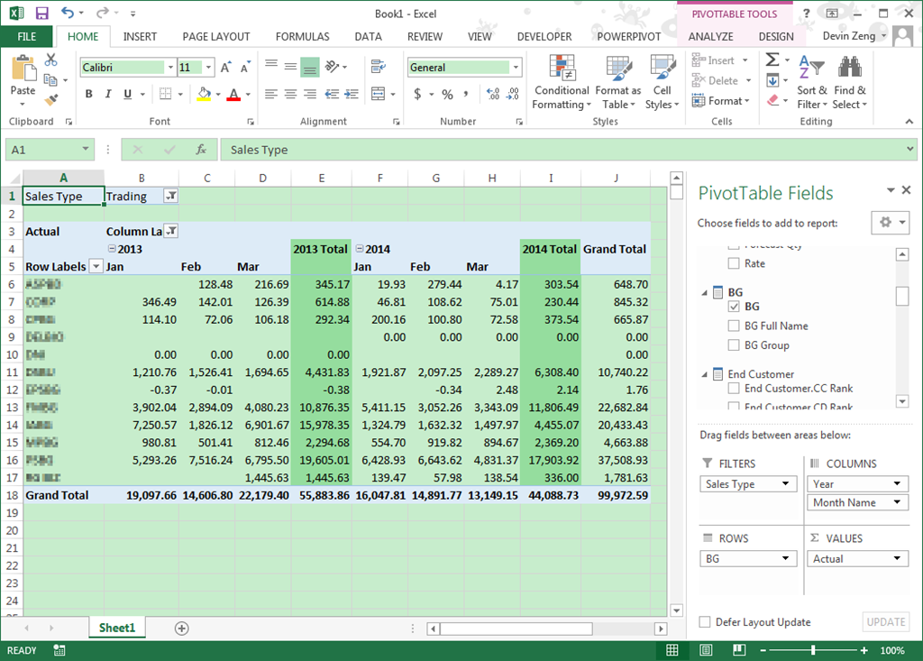
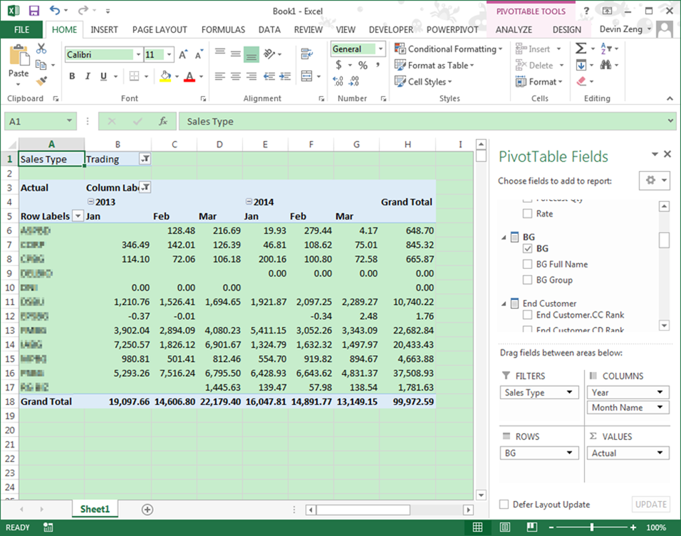
For example, we need display 2013-2014 first quarter every month every BG trading value, we need adjust our pivot table fields like this:
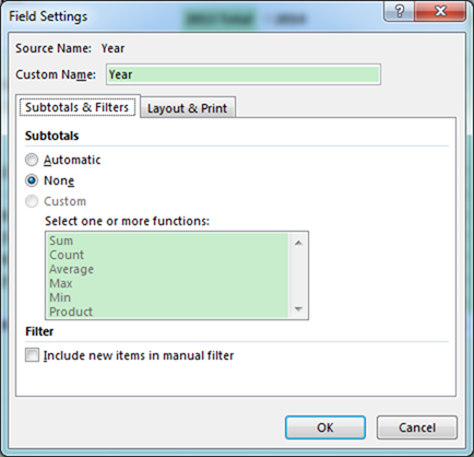
If we don’t want display every year subtotal value, we need find “Year” field on Column panel, click this field, select “Field Settings”, Excel will open a Field Settings window.
At the Subtotals & Filters tab, set Subtotals as “None”.
Now, every year subtotal value will not display on main table.
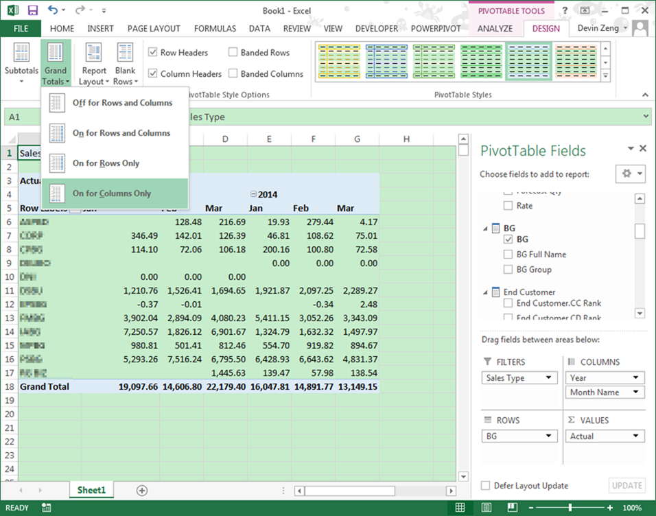
The “Grand Total” column and row also can hide. If we want to hide “H” column grand total, just need display “18” row grand total, click “DESIGN” menu, there is a “Grand Totals” item.
We just need sum every column actual value at the end of the table, so click “On for Columns Only”.
本文转自深蓝居博客园博客,原文链接:http://www.cnblogs.com/studyzy/p/3687801.html,如需转载请自行联系原作者
