Let’s make a DQN 系列
Let’s make a DQN: Theory
1. Theory
2. Implementation
3. Debugging
4. Full DQN
5. Double DQN and Prioritized experience replay (available soon)
Introduction
In February 2015, a group of researches from Google DeepMind published a paper1 which marks a milestone in machine learning. They presented a novel, so called DQN network, which could achieve breathtaking results by playing a set of Atari games, receiving only a visual input.
In these series of articles, we will progressively develop our knowledge to build a state-of-the-art agent, that will be able to learn to solve variety of tasks just by observing the environment. We will explain the needed theoretical background in less technical terms and then build a program to demonstrate how the theory works in practice.
These articles assume some acquaintance with reinforcement learning and artificial neural networks. For those of you, who are not familiar with these terms, I recommend to have a look at a great book from professor Sutton, 19982 first.
We will use Python to program our agent, Keras library to create an artificial neural network (ANN) and OpenAI Gym toolkit as the environment.
Background
The ultimate goal of reinforcement learning is to find a sequence of actions from some state, that lead to a reward. Undoubtedly, some action sequences are better than others. Some sequences might lead to a greater reward, some might get it faster. To develop this idea more, let’s put it down more formally.
The agent is in a state s and has to choose one action a, upon which it receives a reward r and come to a new state s’. The way the agent chooses actions is called policy.

Let’s define a function Q(s, a) such that for given state s and action a it returns an estimate of a total reward we would achieve starting at this state, taking the action and then following some policy. There certainly exist policies that are optimal, meaning that they always select an action which is the best in the context. Let’s call the Q function for these optimal policies Q*.
If we knew the true Q* function, the solution would be straightforward. We would just apply agreedy policy to it. That means that in each state s, we would just choose an action a that maximizes the function Q* – ")
Let’s write a formula for this function in a symbolic way. It is a sum of rewards we achieve after each action, but we will discount every member with γ:
 = r_0 + \gamma r_1 + \gamma^2 r_2 + \gamma^3 r_3 + ...")
γ is called a discount factor and when set it to 
 = r_0 + \gamma (r_1 + \gamma r_2 + \gamma^2 r_3 + ...) = r_0 + \gamma max_a Q^*(s', a)")
We just derived a so called Bellman equation (it’s actually a variation for action values in deterministic environments).
If we turn the formula into a generic assignment  = r + \gamma max_a Q(s', a)")
This is great news. It means that we could use this assignment every time our agent experience a new transition and over time, it would converge to the Q* function. This approach is called online learning and we will discuss it in more detail later.
However, in the problems we are trying to solve, the state usually consists of several real numbers and so our state space is infinite. These numbers could represent for example a position and velocity of the agent or, they could mean something as complex as RGB values of a current screen in an emulator.
We can’t obviously use any table to store infinite number of values. Instead, we will approximate the Q function with a neural network. This network will take a state as an input and produce an estimation of the Q function for each action. And if we use several layers, the name comes naturally – Deep Q-network (DQN).

But the original proof about the convergence does not hold anymore. Actually, the authors of the original research acknowledged that using a neural network to represent the Q function is known to be unstable1. To face with this issue, they introduced several key ideas to stabilize the training, which are mainly responsible for the success we see. Let’s present first of them.
Experience replay
During each simulation step, the agent perform an action a in state s, receives immediate reward r and come to a new state s’. Note that this pattern repeats often and it goes as (s, a, r, s’). The basic idea of online learning is that we use this sample to immediately learn from it.
Because we are using a neural network, we can’t simply use the assignment
but instead, we can shift our estimation towards this target:
 \xrightarrow{} r + \gamma max_a Q(s', a)")
We can do it by performing a gradient descend step with this sample. We intuitively see that by repeating this many times, we are introducing more and more truth into the system and could expect the system to converge. Unfortunately, it is often not the case and it will require some more effort.
The problem with online learning is that the samples arrive in order they are experienced and as such are highly correlated. Because of this, our network will most likely overfit and fail to generalize properly.
The second issue with online learning is that we are not using our experience effectively. Actually, we throw away each sample immediately after we use it.
The key idea of experience replay5 is that we store these transitions in our memory and during each learning step, sample a random batch and perform a gradient descend on it. This way we solve both issues.
Lastly, because our memory is finite, we can typically store only a limited number of samples. Because of this, after reaching the memory capacity we will simply discard the oldest sample.
Exploration
If we always followed the greedy policy, we might never find out that some actions are better then others. A simple technique to resolve this is called ε-greedy policy. This policy behaves greedily most of the time, but chooses a random action with probability ε.
The interesting fact here is that using the previously introduced update formula still shifts the estimated Q function towards the optimal Q* function, even if we use ε-greedy policy to acquire new experience. This is caused by the max in the formula. Because we are not learning the Q function for the policy we are using, but Q* instead, the method is called to beoff-policy.
Implementation
Is it enough to get us started? An earlier research6 shows us it is. In the next chapter, we will implement a simple Q-network that will solve a famous cart-pole problem.
Jaromír Janisch has graduated in 2012 as a Software Engineer from University of West Bohemia. Until 2016 he worked in several software companies, mainly as a developer. He’s been always passionate about progress in artificial intelligence and decided to join the field as a researcher. He is currently preparing to start his Ph.D. studies.
In this blog he strives to extract main points from sometimes complicated scientific research, reformulate them in his own words and make it more accessible for people outside the field.
- Mnih et al. – Human-level control through deep reinforcement learning, Nature 518, 2015
- Sutton R. and Barto A. – Reinforcement Learning: An Introduction, MIT Press, 1998
- Watkins Ch. – Learning from delayed rewards, PhD. thesis, Cambridge University, 1989
- Watkins Ch. and Dayan P. – Q-learning, Machine Learning 8, 1992
- Lin L. – Reinforcement Learning for Robots Using Neural Networks, PhD. thesis, Carnegie Mellon University Pittsburgh, 1993
- Mnih et al. – Playing Atari with Deep Reinforcement Learning, arXiv:1312.5602v1, 2013
Let’s make a DQN: Debugging
1. Theory
2. Implementation
3. Debugging
4. Full DQN
5. Double DQN and Prioritized experience replay (available soon)
Introduction
Last time we saw that our Q-learning can be unstable. In this article we will cover some methods that will help us to understand what is going on inside the network.
The code for this article can be found at github.
Problem
For this article we will choose a different environment – MountainCar-v0, which looks like this:

The goal is to get a car to a flag, which can be seen on the right. The car has to get from the valley, represented by the black line, by accumulating enough momentum. The task is always the same, although the starting position of the car changes with each episode.
The state is represented by only two variables – position and speed of the car. For every time step, the agent receives a reward of -1, until it reaches its goal. There are two actions – push the car left or right.
In MountainCar environment, the agent is continuously penalized and it has to finish the episode as quickly as possible. This is in contrast with the CartPole environment, where the agent accumulated positive reward and tried to prolong the episode for as long as possible.
The simplicity of state space, which is only two dimensional, will allow us to represent it in a human readable way.
Implementation
The coded made in the last article is robust enough to cover also this problem, with only slight changes. However, some improvements and additions were made.
Initialization with random agent
In the beginning of the learning, the agent has an empty memory and also does not know yet what actions to take. We can assume, that a random policy would do the same job in choosing actions, but at much higher rate. Therefore we can simply fill the memory of the agent before the start of the learning itself with a random policy.
Test made with random policy showed that it finishes the episode approximately after 14 000 steps. With memory capacity of 100 000 steps, the agent starts its learning with about 7 episodes of data. This will typically speed up the learning process.
Action reduction
The original OpenGym environment has three actions – push left, do-nothing and ush right. Thedo-nothing action is not needed for solving the problem and will only make the learning more difficult. The point of this article is to demonstrate debugging techniques and this added complexity is not needed. Therefore the actions were remapped so that the do-nothing action is not used.
Hyperparameters
All of the parameters stay the same, except for εmin, which was raised to 0.1.
Normalization
Tests showed that normalizing states doesn’t give any substantial advantage in this problem. However, if we normalize every state variable into [-1 1] region, it allows us to display them in a simple way later.
Debugging
Q function visualization
The network inside the agent is learning a Q function. Let’s recall what this function means. It is an estimate of a discounted total reward the agent would achieve starting in position s and taking action a. The true function also satisfies a property:
So, it is desirable that we understand how this function looks and what it means.
Right from the start we can estimate its range. In this problem the agent always receives a reward of -1 whatever action it takes. At the end of the episode the transition goes straight to the terminal state, for which the Q function is known:
 = r")
Reward r is in this case -1 and at the same time it is the upper bound. In all other non-terminal states it will be lesser than -1.
If we have a minimal sequence of actions leading to a terminal state, starting at a state s and taking a first action a, the value of the Q(s, a) would be:

For an infinite sequence, this gives us the lower bound:

The range of the Q function for all states and actions is therefore:
 \leq -1")
We can now pick pick several points in the Q function and track their values, as the learning progresses. Points of particular interest are at the start and at just before the end of an episode.
By using a trained agent I generated an episode which lasted for 91 steps. Let’s pick these four particular states from it:
|
1
2
3
4
5
|
[
-
0.15955113
,
0.
]
# s_start
[
0.83600049
,
0.27574312
]
# s'' -> s'
[
0.85796947
,
0.28245832
]
# s' -> s
[
0.88062271
,
0.29125591
]
# s -> terminal
|
The correct action in the last three states is to push right, so let’s pick this action and track the Q function at these points. We can do this by simply by calling brain.predict(states).
The expected values at s is -1 and with each step backwards it decreases. We can compute an approximate value for sstart using the formula above to be about -60. The expected values are summarized below:
|
1
2
3
4
|
Q(s, right)
=
-
1
Q(s', right)
=
-
1.99
Q(s'', right)
=
-
2.97
Q(s_start, right) ~
-
60
|
The following graph shows a single run of the algorithm, with the values of the estimated Q function tracked every 1000 steps. Each line correspond to one point in the Q function:
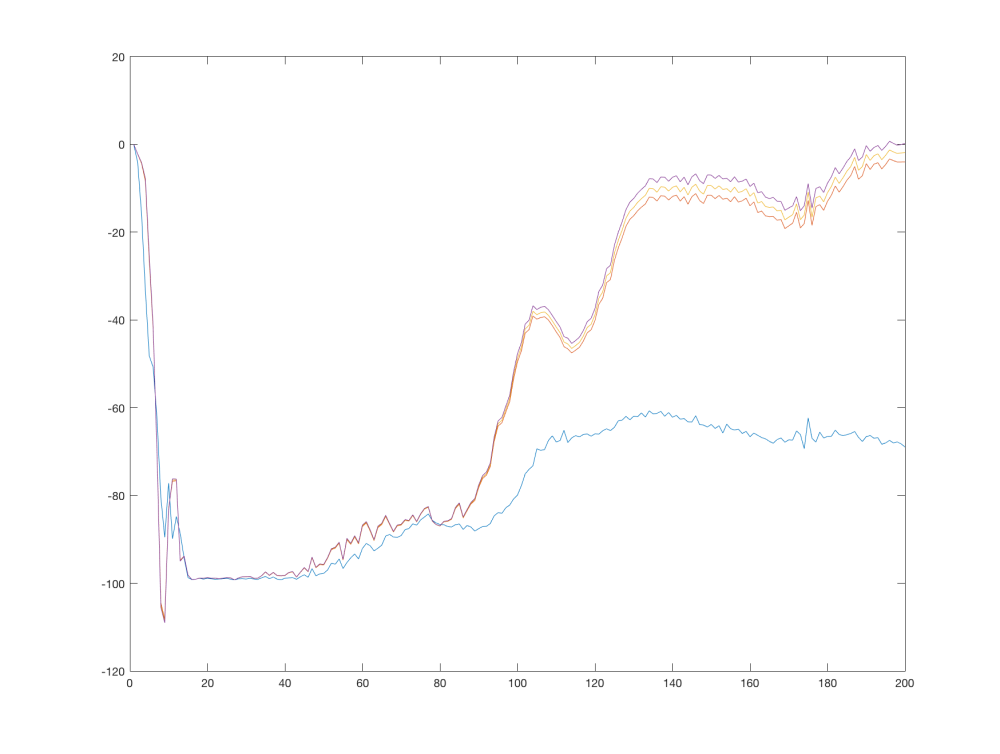
We see that the values start at 0, quickly descending to the minimum of 100. When the learning stabilizes, the terminal transitions start to influence the estimated Q function and this information starts to propagate to other states. After 200 000 steps the Q function values at the tracked points resembles our hand-made estimates. Which line correspond to which point is clear when compared to our estimates.
When we look at the learning after 1 500 000 steps, the chart looks like this:
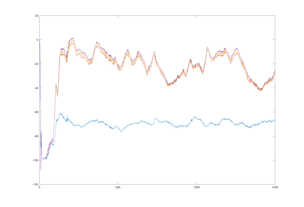
We see that the values oscillate, but keep their relative distance and always tend to return to their true values. This might happen due to several reasons, which we will discuss later.
Value function visualization
Similar to Q function is a value function v(s). It’s defined as a total discounted reward starting at state s and following some policy afterwards. With a greedy policy we can write the value function in terms of the Q function:
 = max_a Q(s, a)")
Because a state in our problem is only two dimensional, it can be visualized as a 2D color map. To more augment this view, we can add another map, showing actions with highest value at a particular point.
We can extract these values from our network by simple forward pass for each point in our state space, with some resolution. Because we normalized our states to be in [-1 1] range, the corresponding states falls to a [-1 1 -1 1] rectangle.
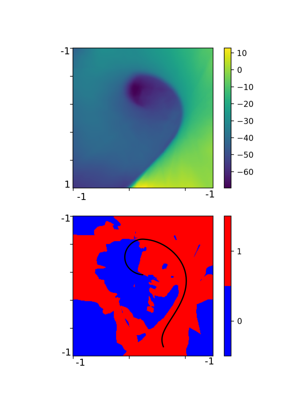
Using a neural network with one hidden layer consisting of 64 neurons, we can generate the following image. It shows both of our maps.

The upper part is a color map of the value function and the bottom part shows areas where the Q function is higher for left (0 or blue) or right (1 or red) action. The vertical axis corresponds to car position and the horizontal axis corresponds to car velocity. The black line shows a trajectory the agent took in a single sample episode.
From the bottom part we can see that the agent did a very good job in generalizing what action to take in which state. The distinction between the two actions is very clear and seems reasonable. The right part of the map corresponds to high speed towards the right of the screen. In these cases the agent always chooses to push more right, because it will likely hit the goal.
Let’s recall how the environment looks like:
The top part in the map corresponds to position on the left slope, from which the agent can gain enough momentum to overcome the slope on the right, reaching the goal. Therefore the agent chooses the push right action.
The blue area corresponds to points where the agent has to get on the left slope first, by choosing the push left action.
The value function itself seems to be correct – the lowest values are in the center, where the agent has no momentum and will likely spend most time getting it, with it’s value raising towards the right and bottom part, corresponding to high right velocity, and position closer to the goal.
However, the right top and bottom corners greater than -1 and are out of the predicted range. This is probably because these states (on the slope left and high right velocity and on the slope right and high right velocity) are never encountered during the learning. Most likely it’s not a problem.
Comparing to high order network
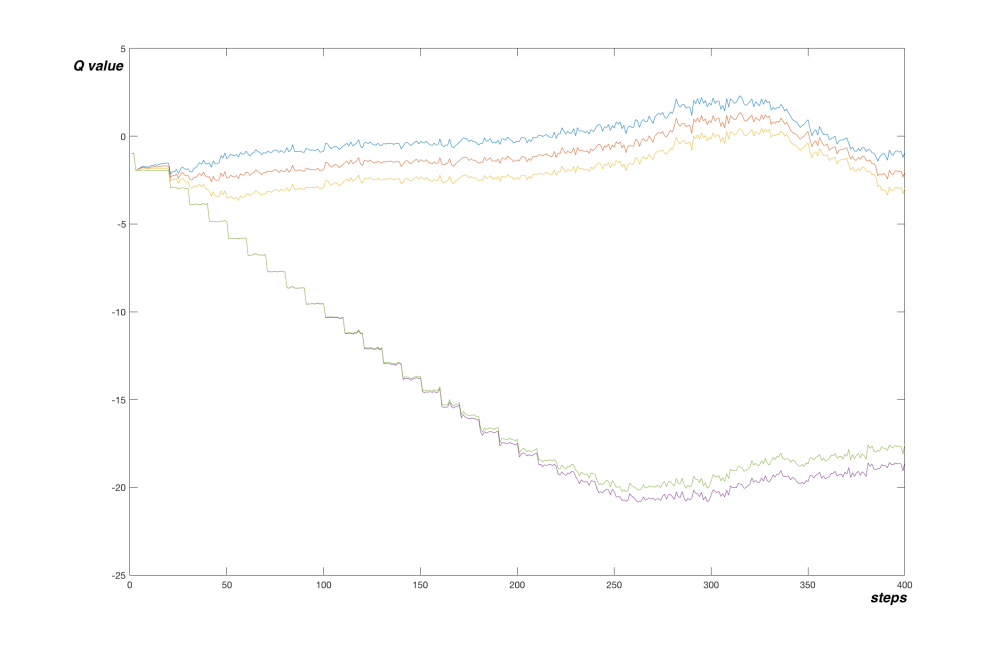
Looking at the value function itself, it seems to be a little fuzzy. It’s unprobable that the true value function is that smooth in all directions. A more sophisticated network could possibly learn a better approximation. Let’s use a network with two hidden layers, each consisting of 256 neurons. First, let’s look at the Q function values graph at the same points as before:
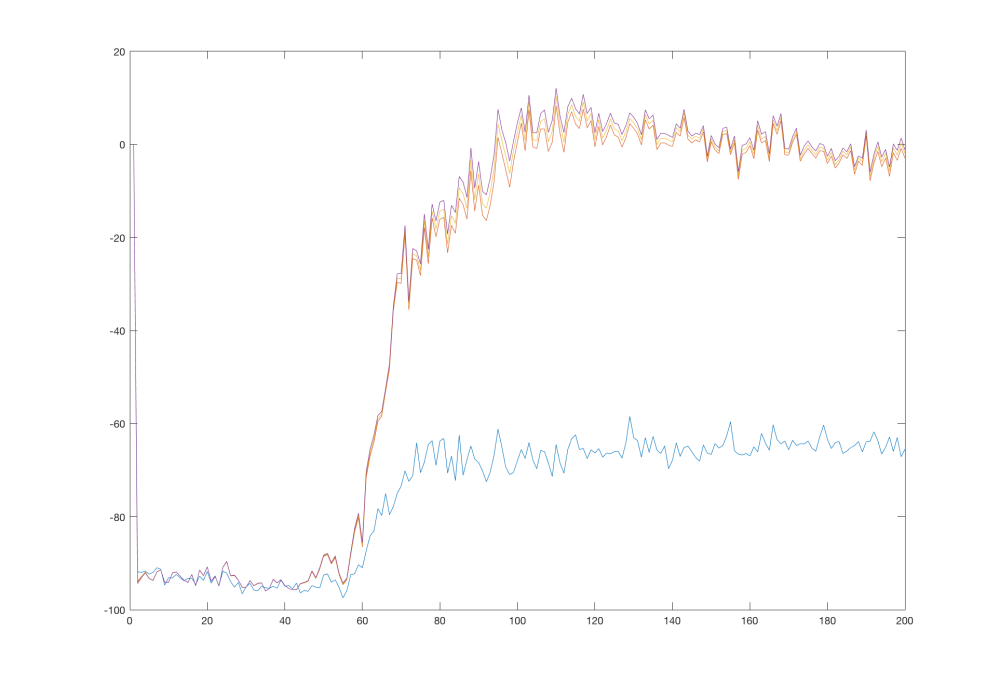
Interestingly, the network converged to the true values quicker than its weaker version. But what is more surprising is that it managed to hold its values around the true values:
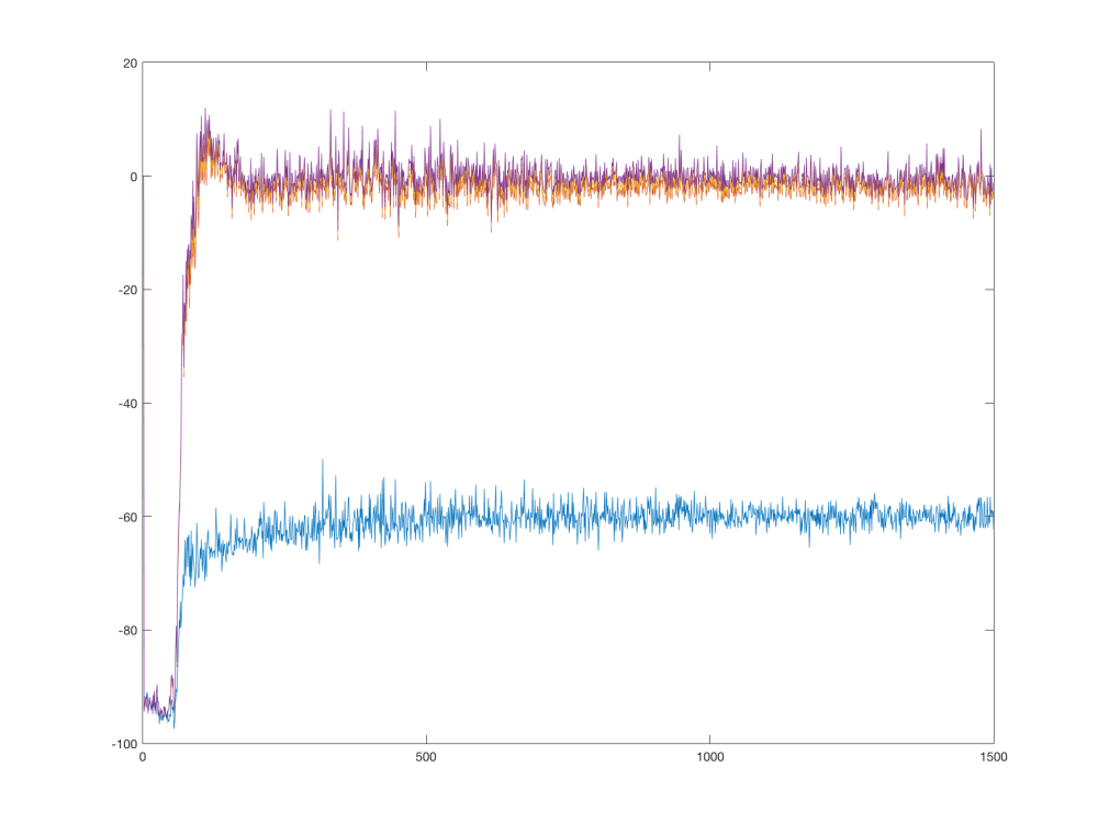
Counterintuitively, the higher order network seems to be more stable. Let’s look at the value function visualization:
At a first glance we can see that the approximation of the value function is much better. However, the action map is a little overcomplicated.
For example, the blue spots on the right, although probably never met in the simulation, are most likely to be incorrect. It seems that our network overfit the training samples and failed to generalize properly beyond them. This also explains the higher speed of convergence and sustained values – the network with many more parameters can accommodate more of specific values easily, but cannot generalize well for values nearby.
We can now conclude that the previous oscillations in the simpler network might have been caused by its insufficient capability to incorporate all the knowledge. Different training samples pull the network in different directions and it unable to satisfy all of them, leading to oscillations.
CartPole revisited
Let’s go back and look at the previous problem – the CartPole environment. We noticed, that its performance suffered several drops, but were unable to say why. With our current knowledge we can plot a joint graph of the reward and a point at the Q function. The point is chosen to be around a sustainable upward position, therefore the agent could theoretically hold the pole upwards indefinitely starting at this state. The true value of the Q function at this state can be computed as 
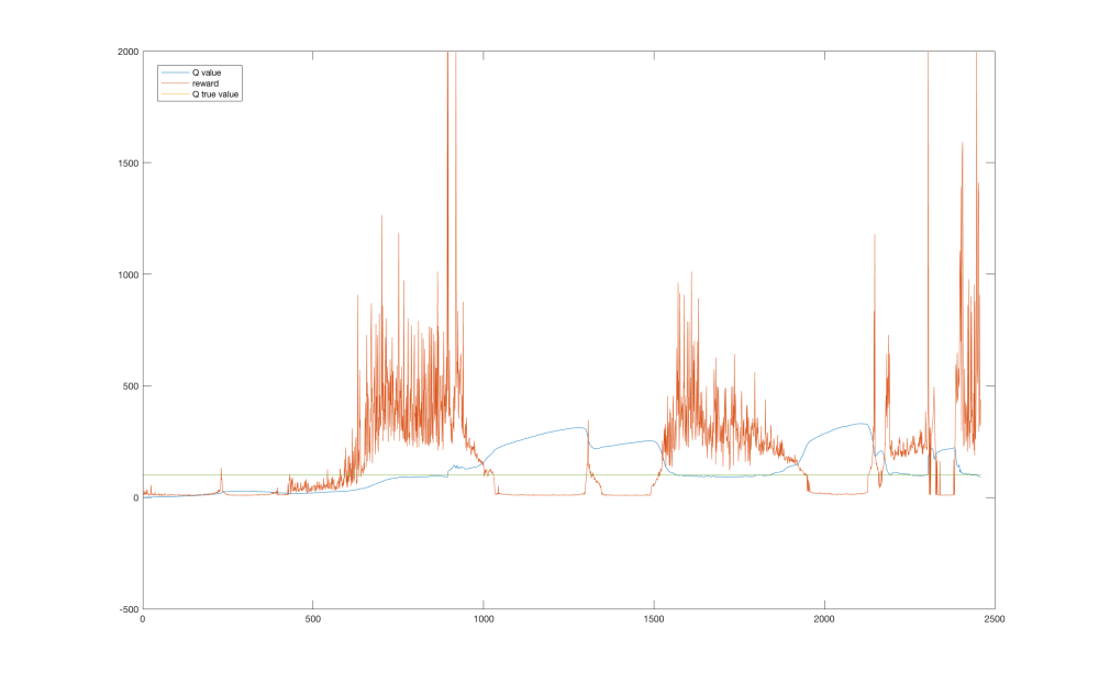
Looking at the graph we can see that the performance drops highly correspond to areas where the value function was overestimated. This could be caused by maximization bias and insufficient exploration.
Reasons of instability
We have identified a few reasons for Q-learning instability. We will now present them briefly, along with other not discussed here and leave thorough discussion to another articles.
Unappropriate network size
We saw that a small network may fail to approximate the Q function properly, whereas a large network can lead to overfitting. Careful network tuning of a network size along with other hyper-parameters can help.
Moving targets
Target depends on the current network estimates, which means that the target for learning moves with each training step. Before the network has a chance to converge to the desired values, the target changes, resulting in possible oscillation or divergence. Solution is to use a fixed target values, which are regularly updated1.
Maximization bias
Due to the max in the formula for setting targets, the network suffers from maximization bias, possibly leading to overestimation of the Q function’s value and poor performance. Double learning can help2.
Outliers with high weight
When a training is performed on a sample which does not correspond to current estimates, it can change the network’s weights substantially, because of the high loss value in MSE loss function, leading to poor performance. The solution is to use a loss clipping1 or a Hubert loss function.
Biased data in memory
If the memory contain only some set of data, the training on this data can eventually change the learned values for important states, leading to poor performance or oscillations. During learning, the agent chooses actions according to its current policy, filling its memory with biased data. Enough exploration can help.
Possible improvements
There are also few ideas how to improve the Q-learning itself.
Priority experience replay
Randomly sampling form a memory is not very efficient. Using a more sophisticated sampling strategy can speed up the learning process3.
Utilizing known truth
Some values of the Q function are known exactly. These are those at the end of the episode, leading to the terminal state. Their value is exactly  = r")
Conclusion
We saw two methods that help us to analyze the Q-learning process. We can display the estimated Q function in known points in a form of graph and we can display a map of a value function in a color map, along with a action map.
We also saw what are some of the reasons of Q-learning instability and possible improvements. In the next article we will make a much more stable solution based on a full DQN network.
Jaromír Janisch has graduated in 2012 as a Software Engineer from University of West Bohemia. Until 2016 he worked in several software companies, mainly as a developer. He’s been always passionate about progress in artificial intelligence and decided to join the field as a researcher. He is currently preparing to start his Ph.D. studies.
In this blog he strives to extract main points from sometimes complicated scientific research, reformulate them in his own words and make it more accessible for people outside the field.
- Mnih et al. – Human-level control through deep reinforcement learning, Nature 518, 2015
- Hasselt et al. – Deep Reinforcement Learning with Double Q-learning, arXiv:1509.06461, 2015
- Schaul et al. – Prioritized Experience Replay, arXiv:1511.05952, 2015
Let’s make a DQN: Full DQN
1. Theory
2. Implementation
3. Debugging
4. Full DQN
5. Double DQN and Prioritized experience replay (available soon)
Introduction
Up until now we implemented a simple Q-network based agent, which suffered from instability issues. In this article we will address these problems with two techniques – target network and error clipping. After implementing these, we will have a fully fledged DQN, as specified by the original paper1.
Target Network
During training of our algorithm we set targets for gradient descend as:
We see that the target depends on the current network. A neural network works as a whole, and so each update to a point in the Q function also influences whole area around that point. And the points of Q(s, a) and Q(s’, a) are very close together, because each sample describes a transition from s to s’. This leads to a problem that with each update, the target is likely to shift. As a cat chasing its own tale, the network sets itself its targets and follows them. As you can imagine, this can lead to instabilities, oscillations or divergence.
To overcome this problem, researches proposed to use a separate target network for setting the targets. This network is a mere copy of the previous network, but frozen in time. It provides stable 
 \xrightarrow{} r + \gamma max_a \tilde{Q}(s', a)")
After severals steps, the target network is updated, just by copying the weights from the current network. To be effective, the interval between updates has to be large enough to leave enough time for the original network to converge.
A drawback is that it substantially slows down the learning process. Any change in the Q function is propagated only after the target network update. The intervals between updated are usually in order of thousands of steps, so this can really slow things down.
On the graph below we can see an effect of a target network in MountainCar problem. The values are plotted every 1000 steps and target network was updated every 10000 steps. We can see the stair-shaped line, where the network converged to provided target values. Each drop corresponds to an update of the target network.
The network more or less converged to true values after 250 000 steps. Let’s look at a graph of a simple Q-network from last article (note that tracked Q function points are different):
Here the algorithm converged faster, after only 100 000 steps. But the shape of the graph is very different. In the simple Q-network variant, the network went fast to the minimum of -100 and started picking the final transitions to reach true values after a while. The algorithm with target network on the other hand quickly anchored the final transitions to their true values and slowly propagated this true value further to the network.
Another direct comparison can be done on the CartPole problem, where the differences are clear:

The version with target network smoothly aim for the true value whereas the simple Q-network shows some oscillations and difficulties.
Although sacrificing speed of learning, this added stability allows the algorithm to learn correct behaviour in much complicated environments, such as those described in the original paper1 – playing Atari games receiving only visual input.
Error clipping
In the gradient descend algorithm, usually Mean Squared Error (MSE) loss function is used. It is defined as:
^2")
where 

^2")
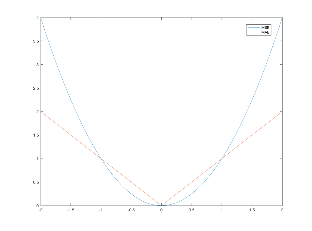
By choosing a different loss function, we can smooth these changes. In the original paper1, clipping of the derivative of MSE to [-1 1] is proposed. This effectively means that MSE is used for errors in the [-1 1] region and Mean Absolute Error (MAE) outside. MAE is defined as:

The differences between the two functions are shown in the following image:
There’s actually a different way of describing such a loss function, in a single quotation. It’s called Huber loss and is defined as

and looks like this:
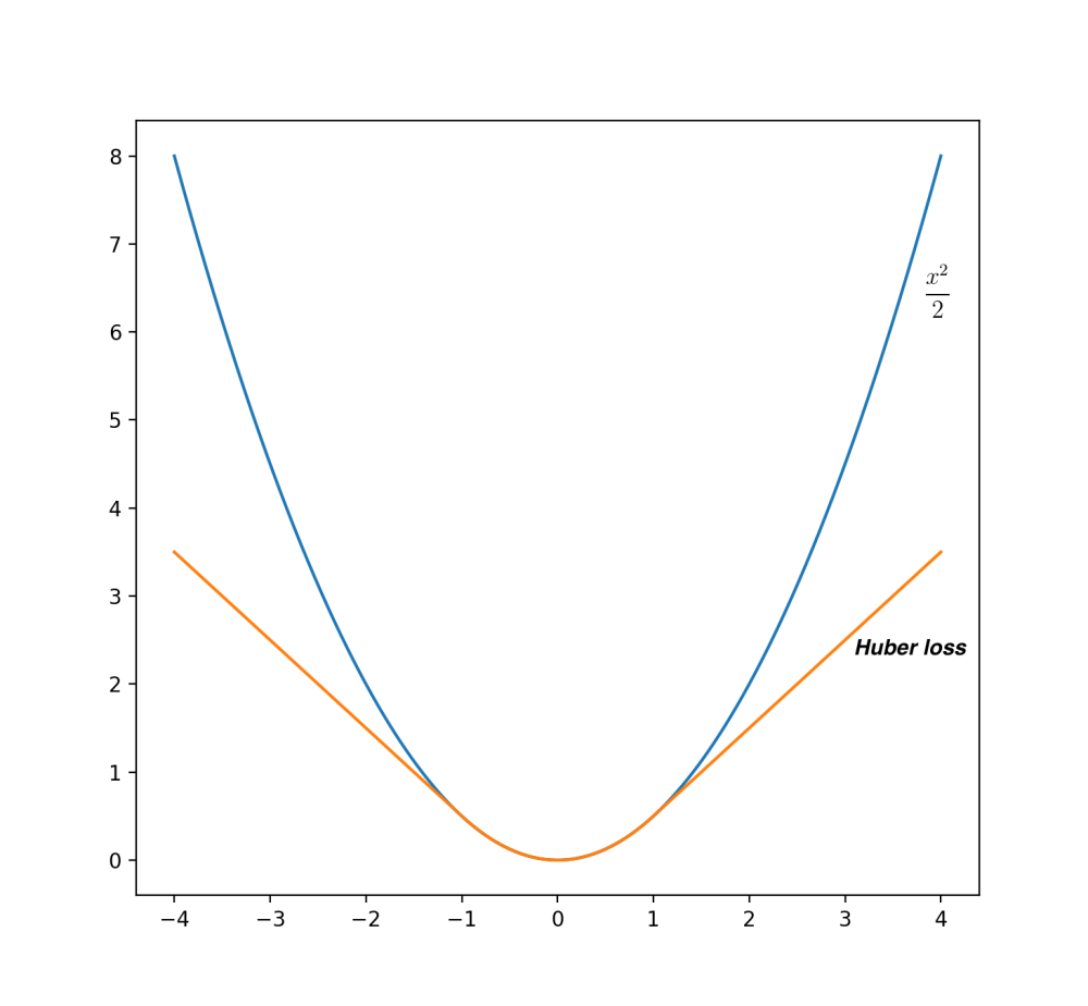
It behaves as 
[-1 1] region and as 
However, the error clipping technique have its drawbacks. It it important to realize that in the back-propagation algorithm, its derivative is actually used. Outside [-1 1] region, the derivative is either -1 or 1 and therefore all errors outside this region will get fixed slowly and at the same constant rate. In some settings this can cause problems. For example in theCartPole environment, the combination of simple Q-network and Huber loss actually systematically caused the network to diverge.
Implementation
You can download a demonstration of DQN on the CartPole problem from github.
The only changes against the old versions are that the Brain class now contains two networksmodel and model_ and we use the target network in the replay() function to get the targets. Also, the initialization with random agent is now used.
Let’s look at the performance. In the following graph, you can see smoothed reward, along with the estimated Q value in one point. Values were plotted every 1000 steps.

We see that the Q function estimate is much more stable than in the simple Q-learning case. The reward tend to be stable too, but at around step 2 200 000, the reward reached an astronomical value of 69628.0, after which the performance dropped suddenly. I assume this is caused by limited memory and experience bias. During this long episode, almost whole memory was filled with highly biased experience, because the agent was holding the pole upright, never experiencing any other state. The gradient descend optimized the network using only this experience and while doing so destroyed the previously learned Q function as a whole.
Conclusion
This article explained the concepts of target network and error clipping, which together with Q-learning form full DQN. We saw how these concepts make learning more stable and offered a reference implementation.
Next time we will look into further improvements, by using Double learning and Prioritized Experience Replay.
Jaromír Janisch has graduated in 2012 as a Software Engineer from University of West Bohemia. Until 2016 he worked in several software companies, mainly as a developer. He’s been always passionate about progress in artificial intelligence and decided to join the field as a researcher. He is currently preparing to start his Ph.D. studies.
In this blog he strives to extract main points from sometimes complicated scientific research, reformulate them in his own words and make it more accessible for people outside the field.
- Mnih et al. – Human-level control through deep reinforcement learning, Nature 518, 2015
Let’s make a DQN: Implementation
1. Theory
2. Implementation
3. Debugging
4. Full DQN
5. Double DQN and Prioritized experience replay (available soon)
Introduction
Last time we tried to get a grasp of necessary knowledge and today we will use it to build an Q-network based agent, that will solve a cart pole balancing problem, in less than 200 lines of code.
The complete code is available at github.
The problem looks like this:

There’s a cart (represented by the black box) with attached pole, that can rotate around one axis. The cart can only go left or right and the goal is to balance the pole as long as possible.
The state is described by four values – cart position, its velocity, pole angle and its angular velocity. At each time step, the agent has to decide whether to push the cart left or right.
If the pole is up, above a certain angle, the agent receives a reward of one. If it falls below this critical angle, the episode ends.
The important fact here is that the agent does not know any of this and has to use its experience to find a viable way to solve this problem. The algorithm is just given four numbers and has to correlate them with the two available actions to acquire as much reward as possible.
Prerequisites
Our algorithm won’t be resource demanding, you can use any recent computer with Python 3 installed to reproduce results in this article. There are some libraries that you have to get before we start. You can install them easily with pip command:
|
1
|
pip
install
theano keras gym
|
This will fetch and install Theano, a low level library for building artificial neural networks. But we won’t use it directly, instead we will use Keras as an abstraction layer. It will allow us to define our ANN in a compact way. The command also installs OpenAI Gym toolkit, which will provide us with easy to use environments for our agent.
The Keras library uses by default TensorFlow, which is a different library from Theano. To switch to Theano, edit ~/.keras/keras.json file so it contains this line:
|
1
|
"backend": "theano",
|
Implementation
Before we jump on to the code itself, let’s think about our problem in an abstract way. There’s an agent, which interacts with the environment through actions and observations. The environment reacts to agent’s actions and supply information about itself. The agent will store the encountered experience in its memory and use its (artificial) intelligence to decide what actions to take. The next diagram shows an abstraction of the problem:
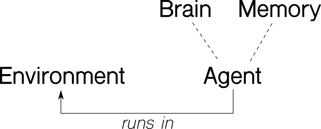
Following our intuition, we will implement four classes – Environment, Agent, Brain andMemory, with these methods:
|
1
2
3
4
5
6
7
8
9
10
11
12
13
14
15
|
Environment
run()
# runs one episode
Agent
act(s)
# decides what action to take in state s
observe(sample)
# adds sample (s, a, r, s_) to memory
replay()
# replays memories and improves
Brain
predict(s)
# predicts the Q function values in state s
train(batch)
# performs supervised training step with batch
Memory
add(sample)
# adds sample to memory
sample(n)
# returns random batch of n samples
|
With this picture in mind, let’s look at each of these in more detail.
Environment
The Environment class is our abstraction for OpenAI Gym. Its only method run() handles one episode of the problem. Look at an excerpt from the run() function:
|
1
2
3
4
5
6
7
8
9
10
11
12
13
14
15
|
s
=
env.reset()
while
True
:
a
=
agent.act(s)
s_, r, done, info
=
env.step(a)
if
done:
s_
=
None
agent.observe( (s, a, r, s_) )
agent.replay()
s
=
s_
if
done:
break
|
In the main loop, the agent decides what action to take, based on given state. The environment then performs this action and returns a new state and a reward.
We will mark the end of the episode by setting the new state s_ to None. The actual state is not needed because there is one terminal state.
Then the agent observes the new sample (s, a, r, s’) and performs a learning step.
Brain
The Brain class encapsulates the neural network. Our problem is simple enough so we will use only one hidden layer of 64 neurons, with ReLU activation function. The final layer will consist of only two neurons, one for each available action. Their activation function will be linear. Remember that we are trying to approximate the Q function, which in essence can be of any real value. Therefore we can’t restrict the output from the network and the linear activation works well.
Instead of simple gradient descend, we will use a more sophisticated algorithm RMSprop, and Mean Squared Error (mse) loss function.
Keras library allows us to define such network surprisingly easily:
|
1
2
3
4
5
6
7
|
model
=
Sequential()
model.add(Dense(output_dim
=
64
, activation
=
'relu'
, input_dim
=
stateCount))
model.add(Dense(output_dim
=
actionCount, activation
=
'linear'
))
opt
=
RMSprop(lr
=
0.00025
)
model.
compile
(loss
=
'mse'
, optimizer
=
opt)
|
The train(x, y) function will perform a gradient descend step with given batch.
|
1
2
|
def
train(
self
, x, y):
model.fit(x, y, batch_size
=
64
)
|
Finally, the predict(s) method returns an array of predictions of the Q function in given states. It’s easy enough again with Keras:
|
1
2
|
def
predict(
self
, s):
model.predict(s)
|
Memory
The purpose of the Memory class is to store experience. It almost feels superfluous in the current problem, but we will implement it anyway. It is a good abstraction for the experience replay part and will allow us to easily upgrade it to more sophisticated algorithms later on.
The add(sample) method stores the experience into the internal array, making sure that it does not exceed its capacity. The other method sample(n) returns n random samples from the memory.
Agent
Finally, the Agent class acts as a container for the agent related properties and methods. The act(s) method implements the ε-greedy policy. With probability epsilon, it chooses a random action, otherwise it selects the best action the current ANN returns.
|
1
2
3
4
5
|
def
act(
self
, s):
if
random.random() <
self
.epsilon:
return
random.randint(
0
,
self
.actionCnt
-
1
)
else
:
return
numpy.argmax(
self
.brain.predictOne(s))
|
We decrease the epsilon parameter with time, according to a formula:
 e^{-\lambda t}")
The λ parameter controls the speed of decay. This way we start with a policy that explores greatly and behaves more and more greedily over time.
The observe(sample) method simply adds a sample to the agent’s memory.
|
1
2
|
def
observe(
self
, sample):
# in (s, a, r, s_) format
self
.memory.add(sample)
|
The last replay() method is the most complicated part. Let’s recall, how the update formula looks like:
This formula means that for a sample (s, r, a, s’) we will update the network’s weights so that its output is closer to the target.
But when we recall our network architecture, we see, that it has multiple outputs, one for each action.
We therefore have to supply a target for each of the outputs. But we want to adjust the ouptut of the network for only the one action which is part of the sample. For the other actions, we want the output to stay the same. So, the solution is simply to pass the current values as targets, which we can get by a single forward propagation.
Also, we have a special case of the episode terminal state. Remember that we set a state toNone in the Environment class when the episode ended. Because of that, we can now identify such a state and act accordingly.
When the episode ends, there are no more states after and so our update formula reduces to
 \xrightarrow{} r")
In this case, we will set our target only to r.
Let’s look at the code now. First we fetch a batch of samples from the memory.
|
1
|
batch
=
self
.memory.sample(BATCH_SIZE)
|
We can now make the predictions for all starting and ending states in our batch in one step. The underlaying Theano library will parallelize our code seamlessly, if we supply an array of states to predict. This results to a great speedup.
|
1
2
3
4
5
6
7
|
no_state
=
numpy.zeros(
self
.stateCnt)
states
=
numpy.array([ o[
0
]
for
o
in
batch ])
states_
=
numpy.array([ (no_state
if
o[
3
]
is
None
else
o[
3
])
for
o
in
batch ])
p
=
agent.brain.predict(states)
p_
=
agent.brain.predict(states_)
|
Notice the no_state variable. We use it as a dummy replacement state for the occasions where the final state is None. The Theano librarary cannot make a preditiction for a None state, therefore we just supply an array full of zeroes.
The p variable now holds predictions for the starting states for each sample and will be used as a default target in the learning. Only the one action passed in the sample will have the actual target of ")
The other p_ variable is filled with predictions for the final states and is used in the ")
We now iterate over all the samples and set proper targets for each sample:
|
1
2
3
4
5
6
7
8
9
10
11
12
|
for
i
in
range
(batchLen):
o
=
batch[i]
s
=
o[
0
]; a
=
o[
1
]; r
=
o[
2
]; s_
=
o[
3
]
t
=
p[i]
if
s_
is
None
:
t[a]
=
r
else
:
t[a]
=
r
+
GAMMA
*
numpy.amax(p_[i])
x[i]
=
s
y[i]
=
t
|
Finally, we call our brain.train() method:
|
1
|
self
.brain.train(x, y)
|
Main
To make our program more general, we won’t hardcode state space dimensions nor number of possible actions. Instead we retrieve them from the environment. In the main loop, we just run the episodes forever, until the user terminates with CTRL+C.
|
1
2
3
4
5
6
7
8
9
10
|
PROBLEM
=
'CartPole-v0'
env
=
Environment(PROBLEM)
stateCnt
=
env.env.observation_space.shape[
0
]
actionCnt
=
env.env.action_space.n
agent
=
Agent(stateCnt, actionCnt)
while
True
:
env.run(agent)
|
Normalization
Although a neural network can in essence adapt to any input, normalizing it will typically help. We can sample a few examples of different states to see what they look like:
|
1
2
3
4
|
[-0.0048 0.0332 -0.0312 0.0339]
[-0.01 -0.7328 0.0186 1.1228]
[-0.166 -0.4119 0.1725 0.8208]
[-0.0321 0.0445 0.0284 -0.0034]
|
We see that they are essentially similar in their range, and their magnitude do not differ substantially. Because of that, we won’t normalize the input in this problem.
Hyperparameters
So far we talked about the components in a very generic way. We didn’t give any concrete values for the parameters mentioned in previous sections, except for the neural network architecture. Following parameters were chosen to work well in this problem:
| PARAMETER | VALUE |
|---|---|
| memory capacity | 100000 |
| batch size | 64 |
| γ | 0.99 |
| εmax | 1.00 |
| εmin | 0.01 |
| λ | 0.001 |
| RMSprop learning rate | 0.00025 |
Results
You can now download the full code and try it for yourself:
https://github.com/jaara/AI-blog/blob/master/CartPole-basic.py
It’s remarkable that with less than 200 lines of code, we can implement a Q-network based agent. Although we used CartPole-v0 environment as an example, we can use the same code for many different environments, with only small adjustments. Also, our agent runs surprisingly fast. With disabled rendering, it achieves about 720 FPS on my notebook. Now, let’s look how well it actually performs.
The agent usually learns to hold the pole in straight position after some time, with varying accuracy. To be able to compare results, I ran several thousand episodes with a random policy, which achieved an average reward of 22.6. Then I averaged a reward over 10 runs with our agent, each with 1000 episodes with a limit of 2000 time steps:

We see that it is well above the average reward of a random policy, so we can conclude that our agent actually learned something. But these results are averaged over multiple runs and the celebrations would be premature. Let’s look at a single run and its reward:
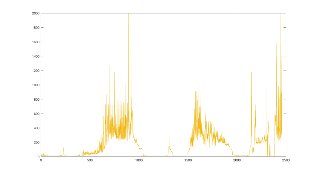
We see that there are several spots where the performance drops suddenly to zero. Clearly, our learning algorithm is unstable. What could be causing these drops and why? Does the network overfit or diverge? Or is it something else? And more importantly, can we mitigate these issues?
As a matter of fact, we can. There are several points in our agent, which we can improve. But before we do that, we have to understand, what the underlaying neural network is doing. In the next section, we will get means to take a meaningful insight into the neural network itself, learn how to display the approximated Q function and use this knowledge to understand what is happening.
Jaromír Janisch has graduated in 2012 as a Software Engineer from University of West Bohemia. Until 2016 he worked in several software companies, mainly as a developer. He’s been always passionate about progress in artificial intelligence and decided to join the field as a researcher. He is currently preparing to start his Ph.D. studies.
In this blog he strives to extract main points from sometimes complicated scientific research, reformulate them in his own words and make it more accessible for people outside the field.
Code :
# OpenGym CartPole-v0
# -------------------
#
# This code demonstrates use of a basic Q-network (without target network)
# to solve OpenGym CartPole-v0 problem.
#
# Made as part of blog series Let's make a DQN, available at:
# https://jaromiru.com/2016/10/03/lets-make-a-dqn-implementation/
#
# author: Jaromir Janisch, 2016


#--- enable this to run on GPU
# import os
# os.environ['THEANO_FLAGS'] = "device=gpu,floatX=float32"

import random, numpy, math, gym

#-------------------- BRAIN ---------------------------
from keras.models import Sequential
from keras.layers import *
from keras.optimizers import *

class Brain:
    def __init__(self, stateCnt, actionCnt):
        self.stateCnt = stateCnt
        self.actionCnt = actionCnt

        self.model = self._createModel()
        # self.model.load_weights("cartpole-basic.h5")

    def _createModel(self):
        model = Sequential()

        model.add(Dense(output_dim=64, activation='relu', input_dim=stateCnt))
        model.add(Dense(output_dim=actionCnt, activation='linear'))

        opt = RMSprop(lr=0.00025)
        model.compile(loss='mse', optimizer=opt)

        return model

    def train(self, x, y, epoch=1, verbose=0):
        self.model.fit(x, y, batch_size=64, nb_epoch=epoch, verbose=verbose)

    def predict(self, s):
        return self.model.predict(s)

    def predictOne(self, s):
        return self.predict(s.reshape(1, self.stateCnt)).flatten()

#-------------------- MEMORY --------------------------
class Memory:   # stored as ( s, a, r, s_ )
    samples = []

    def __init__(self, capacity):
        self.capacity = capacity

    def add(self, sample):
        self.samples.append(sample)

        if len(self.samples) > self.capacity:
            self.samples.pop(0)

    def sample(self, n):
        n = min(n, len(self.samples))
        return random.sample(self.samples, n)

#-------------------- AGENT ---------------------------
MEMORY_CAPACITY = 100000
BATCH_SIZE = 64

GAMMA = 0.99

MAX_EPSILON = 1
MIN_EPSILON = 0.01
LAMBDA = 0.001      # speed of decay

class Agent:
    steps = 0
    epsilon = MAX_EPSILON

    def __init__(self, stateCnt, actionCnt):
        self.stateCnt = stateCnt
        self.actionCnt = actionCnt

        self.brain = Brain(stateCnt, actionCnt)
        self.memory = Memory(MEMORY_CAPACITY)

    def act(self, s):
        if random.random() < self.epsilon:
            return random.randint(0, self.actionCnt-1)
        else:
            return numpy.argmax(self.brain.predictOne(s))

    def observe(self, sample):  # in (s, a, r, s_) format
        self.memory.add(sample)

        # slowly decrease Epsilon based on our eperience
        self.steps += 1
        self.epsilon = MIN_EPSILON + (MAX_EPSILON - MIN_EPSILON) * math.exp(-LAMBDA * self.steps)

    def replay(self):
        batch = self.memory.sample(BATCH_SIZE)
        batchLen = len(batch)

        no_state = numpy.zeros(self.stateCnt)

        states = numpy.array([ o[0] for o in batch ])
        states_ = numpy.array([ (no_state if o[3] is None else o[3]) for o in batch ])

        p = agent.brain.predict(states)
        p_ = agent.brain.predict(states_)

        x = numpy.zeros((batchLen, self.stateCnt))
        y = numpy.zeros((batchLen, self.actionCnt))

        for i in range(batchLen):
            o = batch[i]
            s = o[0]; a = o[1]; r = o[2]; s_ = o[3]

            t = p[i]
            if s_ is None:
                t[a] = r
            else:
                t[a] = r + GAMMA * numpy.amax(p_[i])

            x[i] = s
            y[i] = t

        self.brain.train(x, y)

#-------------------- ENVIRONMENT ---------------------
class Environment:
    def __init__(self, problem):
        self.problem = problem
        self.env = gym.make(problem)

    def run(self, agent):
        s = self.env.reset()
        R = 0

        while True:
            self.env.render()

            a = agent.act(s)

            s_, r, done, info = self.env.step(a)

            if done: # terminal state
                s_ = None

            agent.observe( (s, a, r, s_) )
            agent.replay()

            s = s_
            R += r

            if done:
                break

        print("Total reward:", R)

#-------------------- MAIN ----------------------------
PROBLEM = 'CartPole-v0'
env = Environment(PROBLEM)

stateCnt  = env.env.observation_space.shape[0]
actionCnt = env.env.action_space.n

agent = Agent(stateCnt, actionCnt)

try:
    while True:
        env.run(agent)
finally:
    agent.brain.model.save("cartpole-basic.h5")

![大语言模型的预训练[3]之Prompt Learning:Prompt Engineering、Answer engineering、Multi-prompt learning、Training strategy详解](https://ucc.alicdn.com/pic/developer-ecology/fnj5anauszhew_8ead1a3213f047beb6ba28bc8d7647af.png?x-oss-process=image/resize,h_160,m_lfit)