标签
PostgreSQL , Greenplum , hash outer join , hash table
背景
数据分析、大表JOIN、多表JOIN时,哈希JOIN是比较好的提速手段。
hash join会首先扫描其中的一张表(包括需要输出的字段),根据JOIN列生成哈希表。然后扫描另一张表。
hash join介绍
https://www.postgresql.org/docs/10/static/planner-optimizer.html
the right relation is first scanned and loaded into a hash table, using its join attributes as hash keys.
Next the left relation is scanned and the appropriate values of every row found are used as hash keys to locate the matching rows in the table.
hash table的选择
理论上应该选择小表作为哈希表。但是2011年以前的版本,对HASH表的选择是有讲究的,并不是自由选择,只支OUTER JOIN时返回可以为空的表生成哈希表。
hash join演进
PostgreSQL在1997年的时候已经支持HashJoin,Greenplum基于PostgreSQL 8.2开发,因此也是天然支持HashJoin的。
在2011年时,PostgreSQL对hashjoin做出了两个改进,支持full outer join,同时支持outer join任意表生成哈希表(原来的版本只支OUTER JOIN时返回可以为空的表生成哈希表):
https://www.postgresql.org/docs/current/static/release-9-1.html
Allow FULL OUTER JOIN to be implemented as a hash join, and allow either side of a LEFT OUTER JOIN or RIGHT OUTER JOIN to be hashed (Tom Lane)
Previously FULL OUTER JOIN could only be implemented as a merge join, and LEFT OUTER JOIN and RIGHT OUTER JOIN could hash only the nullable side of the join.
These changes provide additional query optimization possibilities.
对应patch
这个改进非常有意义,特别是可以为空的表非常庞大时,作为哈希表是不合适的。后面就来对比一下。
几种JOIN介绍
INNER JOIN
For each row R1 of T1, the joined table has a row for each row in T2 that satisfies the join condition with R1.
LEFT OUTER JOIN
First, an inner join is performed.
Then, for each row in T1 that does not satisfy the join condition with any row in T2,
a joined row is added with null values in columns of T2.
Thus, the joined table always has at least one row for each row in T1.
RIGHT OUTER JOIN
First, an inner join is performed.
Then, for each row in T2 that does not satisfy the join condition with any row in T1,
a joined row is added with null values in columns of T1.
This is the converse of a left join: the result table will always have a row for each row in T2.
FULL OUTER JOIN
First, an inner join is performed.
Then, for each row in T1 that does not satisfy the join condition with any row in T2,
a joined row is added with null values in columns of T2.
Also, for each row of T2 that does not satisfy the join condition with any row in T1,
a joined row with null values in the columns of T1 is added.
PostgreSQL vs Greenplum outer join 对比
left\right outer join
PostgreSQL 9.1+
postgres=# create table t1(id int, info text);
CREATE TABLE
postgres=# create table t2(id int, info text);
CREATE TABLE

t1为小表, t2为大表

postgres=# insert into t1 select generate_series(1,10000);
INSERT 0 10000
postgres=# insert into t2 select generate_series(1,10000000);
INSERT 0 10000000
postgres=# analyze t1;
ANALYZE
postgres=# analyze t2;
ANALYZE
PostgreSQL自动选择了小表作为哈希表。
postgres=# explain (analyze,verbose,timing,costs,buffers) select t1.*,t2.* from t1 left outer join t2 on (t1.id=t2.id);
                                                          QUERY PLAN
-------------------------------------------------------------------------------------------------------------------------------
 Hash Right Join  (cost=270.00..182117.68 rows=10000 width=72) (actual time=3.367..2736.484 rows=10000 loops=1)
   Output: t1.id, t1.info, t2.id, t2.info
   Hash Cond: (t2.id = t1.id)
   Buffers: shared hit=16260 read=28033 dirtied=7288 written=5780
   ->  Seq Scan on public.t2  (cost=0.00..144247.77 rows=9999977 width=36) (actual time=0.014..1262.472 rows=10000000 loops=1)
         Output: t2.id, t2.info
         Buffers: shared hit=16228 read=28020 dirtied=7288 written=5780
   ->  Hash  (cost=145.00..145.00 rows=10000 width=36) (actual time=3.323..3.323 rows=10000 loops=1)
         Output: t1.id, t1.info
         Buckets: 16384  Batches: 1  Memory Usage: 480kB
         Buffers: shared hit=32 read=13
         ->  Seq Scan on public.t1  (cost=0.00..145.00 rows=10000 width=36) (actual time=0.033..1.501 rows=10000 loops=1)
               Output: t1.id, t1.info
               Buffers: shared hit=32 read=13
 Planning time: 0.076 ms
 Execution time: 2737.441 ms
(16 rows)
Greenplum
greenplum只能选择nullable端的表作为哈希表。即t2.
postgres=# explain analyze select t1.*,t2.* from t1 left outer join t2 on (t1.id=t2.id);
                                                                      QUERY PLAN
-------------------------------------------------------------------------------------------------------------------------------------------------------
 Gather Motion 48:1  (slice1; segments: 48)  (cost=236070.60..236368.60 rows=10000 width=72)
   Rows out:  10000 rows at destination with 215 ms to end, start offset by 1.350 ms.
   ->  Hash Left Join  (cost=236070.60..236368.60 rows=209 width=72)
         Hash Cond: t1.id = t2.id
         Rows out:  Avg 208.3 rows x 48 workers.  Max 223 rows (seg17) with 0.043 ms to first row, 81 ms to end, start offset by 15 ms.
         Executor memory:  6511K bytes avg, 6513K bytes max (seg18).
         Work_mem used:  6511K bytes avg, 6513K bytes max (seg18). Workfile: (0 spilling, 0 reused)
         ->  Seq Scan on t1  (cost=0.00..148.00 rows=209 width=36)
               Rows out:  Avg 208.3 rows x 48 workers.  Max 223 rows (seg17) with 0.006 ms to first row, 0.025 ms to end, start offset by 15 ms.
         ->  Hash  (cost=111053.60..111053.60 rows=208362 width=36)
               Rows in:  (No row requested) 0 rows (seg0) with 0 ms to end.
               ->  Seq Scan on t2  (cost=0.00..111053.60 rows=208362 width=36)
                     Rows out:  Avg 208333.3 rows x 48 workers.  Max 208401 rows (seg18) with 79 ms to first row, 98 ms to end, start offset by 15 ms.
 Slice statistics:
   (slice0)    Executor memory: 283K bytes.
   (slice1)    Executor memory: 250K bytes avg x 48 workers, 250K bytes max (seg0).  Work_mem: 6513K bytes max.
 Statement statistics:
   Memory used: 128000K bytes
 Settings:  optimizer=off
 Optimizer status: legacy query optimizer
 Total runtime: 216.814 ms
(21 rows)
full outer join
PostgreSQL 9.1+
PostgreSQL 9.1+ 支持full outer join使用hash join.
postgres=# explain (analyze,verbose,timing,costs,buffers) select t1.*,t2.* from t2 full outer join t1 on (t1.id=t2.id);
                                                          QUERY PLAN
-------------------------------------------------------------------------------------------------------------------------------
 Hash Full Join  (cost=270.00..182117.68 rows=9999977 width=72) (actual time=3.434..3728.277 rows=10000000 loops=1)
   Output: t1.id, t1.info, t2.id, t2.info
   Hash Cond: (t2.id = t1.id)
   Buffers: shared hit=16301 read=27992
   ->  Seq Scan on public.t2  (cost=0.00..144247.77 rows=9999977 width=36) (actual time=0.246..1187.189 rows=10000000 loops=1)
         Output: t2.id, t2.info
         Buffers: shared hit=16256 read=27992
   ->  Hash  (cost=145.00..145.00 rows=10000 width=36) (actual time=3.157..3.157 rows=10000 loops=1)
         Output: t1.id, t1.info
         Buckets: 16384  Batches: 1  Memory Usage: 480kB
         Buffers: shared hit=45
         ->  Seq Scan on public.t1  (cost=0.00..145.00 rows=10000 width=36) (actual time=0.013..1.438 rows=10000 loops=1)
               Output: t1.id, t1.info
               Buffers: shared hit=45
 Planning time: 0.095 ms
 Execution time: 4527.421 ms
(16 rows)
Greenplum
Greenplum 8.2版本,不支持full outer join使用hash join.
使用了merge join.
postgres=# explain analyze select t1.*,t2.* from t2 full outer join t1 on (t1.id=t2.id);
                                                                        QUERY PLAN
-----------------------------------------------------------------------------------------------------------------------------------------------------------
 Gather Motion 48:1  (slice1; segments: 48)  (cost=1274708.75..1324865.55 rows=10001360 width=72)
   Rows out:  10000000 rows at destination with 2310 ms to end, start offset by 229 ms.
   ->  Merge Full Join  (cost=1274708.75..1324865.55 rows=208362 width=72)
         Merge Cond: t2.id = t1.id
         Rows out:  Avg 208333.3 rows x 48 workers.  Max 208401 rows (seg18) with 0.002 ms to first row, 36 ms to end, start offset by 274 ms.
         ->  Sort  (cost=1273896.37..1298899.77 rows=208362 width=36)
               Sort Key: t2.id
               Rows out:  Avg 208333.3 rows x 48 workers.  Max 208401 rows (seg18) with 0.006 ms to end, start offset by 274 ms.
               Executor memory:  14329K bytes avg, 14329K bytes max (seg0).
               Work_mem used:  14329K bytes avg, 14329K bytes max (seg0). Workfile: (0 spilling, 0 reused)
               ->  Seq Scan on t2  (cost=0.00..111053.60 rows=208362 width=36)
                     Rows out:  Avg 208333.3 rows x 48 workers.  Max 208401 rows (seg18) with 0.003 ms to first row, 67 ms to end, start offset by 274 ms.
         ->  Sort  (cost=812.39..837.39 rows=209 width=36)
               Sort Key: t1.id
               Rows out:  Avg 208.3 rows x 48 workers.  Max 223 rows (seg17) with 0.002 ms to end, start offset by 273 ms.
               Executor memory:  58K bytes avg, 58K bytes max (seg0).
               Work_mem used:  58K bytes avg, 58K bytes max (seg0). Workfile: (0 spilling, 0 reused)
               ->  Seq Scan on t1  (cost=0.00..148.00 rows=209 width=36)
                     Rows out:  Avg 208.3 rows x 48 workers.  Max 223 rows (seg17) with 31 ms to first row, 32 ms to end, start offset by 273 ms.
 Slice statistics:
   (slice0)    Executor memory: 411K bytes.
   (slice1)    Executor memory: 14597K bytes avg x 48 workers, 14597K bytes max (seg0).  Work_mem: 14329K bytes max.
 Statement statistics:
   Memory used: 128000K bytes
 Settings:  optimizer=off
 Optimizer status: legacy query optimizer
 Total runtime: 2539.416 ms
(27 rows)